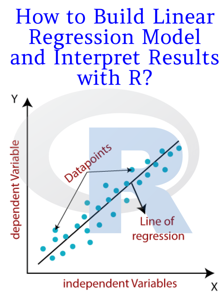
Build Linear Regression Model and Interpret Results with R

Linear regression is a widely used statistical modeling technique for predicting the relationship between a dependent variable and one or more independent variables. It is commonly used in various fields such as economics, finance, marketing, and social sciences. In this article, we will discuss how to build a linear regression model in R and interpret its results.

Download (PDF)

Steps to build a linear regression model in R:

Step 1: Install and load the necessary packages

To build a linear regression model in R, we need to install and load the necessary packages. The “tidyverse” package includes many useful packages, including “dplyr”, “ggplot2”, and “tidyr”. We will also use the “lm” function, which is built into R, for building the linear regression model.

# install.packages("tidyverse")
library(tidyverse)

Step 2: Load and explore the data

We need to load the data into R and explore its structure, dimensions, and summary statistics to gain insights into the data. In this example, we will use the “mtcars” dataset, which is included in R. This dataset contains information about various car models and their performance characteristics.

data(mtcars)
head(mtcars)
summary(mtcars)

Step 3: Create the model

To create the linear regression model, we need to use the “lm” function in R. We need to specify the dependent variable and the independent variables in the formula. In this example, we will use the “mpg” (miles per gallon) variable as the dependent variable and the “wt” (weight) variable as the independent variable.

# Create the linear regression model
model <- lm(mpg ~ wt, data = mtcars)

Step 4: Interpret the model

Once the model is created, we need to interpret its coefficients, standard errors, p-values, and R-squared value to understand its significance and predictive power.

# Display the model coefficients, standard errors, p-values, and R-squared value
summary(model)

The output of the summary() function shows the following:

Call:
lm(formula = mpg ~ wt, data = mtcars)

Residuals:
    Min      1Q  Median      3Q     Max 
-4.5432 -2.3647 -0.1252  1.4096  6.8727 

Coefficients:
            Estimate Std. Error t value Pr(>|t|)    
(Intercept)  37.2851     1.8776  19.858  < 2e-16 ***
wt           -5.3445     0.5591  -9.559 1.29e-10 ***
---
Signif. codes:  0 ‘***’ 0.001 ‘**’ 0.01 ‘*’ 0.05 ‘.’ 0.1 ‘ ’ 1

Residual standard error: 3.046 on 30 degrees of freedom
Multiple R-squared:  0.7528,    Adjusted R-squared:  0.7446 
F-statistic: 91.38 on 1 and 30 DF,  p-value: 1.294e-10

The “Estimate” column shows the coefficients of the linear regression model. The intercept value is 37.2851, which represents the predicted value of the dependent variable when the independent variable is zero. The coefficient of the “wt” variable is -5.3445, which indicates that as the weight of the car increases by one.