excel

You can display your data analysis reports in several ways in Excel. However, if you know the right data visualization technique your data analysis results can be more notable, and your audience can quickly grasp what you want to project in the data. It also leaves a good impact on your presentation style. You can improve your data visualization productivity by using the built-in table functionality available in Excel.

1. Create The Table

Place your cursor in the area you want to make a table. On the menu bar, select Insert, Table.  Excel will guess the range to create the table.

You will then validate the area that Excel has determined is the table you wish to create. Your table should have headers and the checkbox will default to accept the first row of the range to be the table headers.

Once you hit OK the range will format as a table with the default formatting. Select Table Tools that will now be visible on the menu bar which will display more formatting options.

The Design menu bar has many visual and operational options to choose from, some of which we will cover below.

2. Name the Table to Allow for Easier References

As shown in the screen capture above, the default name for the first table is “Table1”. Naming the table something meaningful allows you to reference the table in calculations and other functionality. The reference, rather being Table1 would be YearlySalary which allows for built-in documentation making your calculations more meaningful.

To change the table name, enter a new value in the Table Name box under the Table Tools option on the toolbar, as pictured below.

3. Format the Columns

As you use the tables in other Excel features, such as pivot tables and graphs, the column format will be picked up in the other tools. For example, formatting the columns as Currency and then no decimals will cause the formats to be used in Graphs as shown in the last section below.

4. Insert Slicers

Under the table tools, there is a Slicer option. Clicking on this option allows you to use various columns in the table as filters which allows you to slice the data for different views. With a cell selected in the table, select the Insert Slicer toolbar item in the Table Tools menu bar. You can then select the slicers you want to add.  The final view is below with the Insert Slicer dialogue.

5. Insert a Chart

Now that you have filters you can easily add a chart. Selecting the table, you can insert a graph by selecting the Insert menu option then, select a chart you want to view by selecting that option on the toolbar.  The graph is then filtered based on your slicer selection.

In this day and age, our data dependence is overwhelming. Thanks to our cellphones and laptop, a halo of data surrounds our life. Data is nothing but a piece of classified information. Microsoft Excel is one of the most used data handling/analysis software. At the same time, one tiny mistake in analyzing data can cause headaches. Data is the backbone of any analysis that you do. It is an eternal problem and not only in Excel! Here’s a list of the top 10 Super Neat Ways to Clean Data in Excel as follows.

1. Get Rid of Extra Spaces

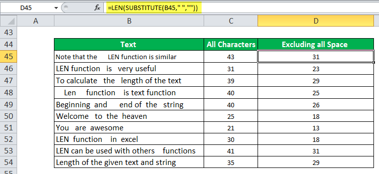
When it comes to clean data on excel extra spaces are painfully difficult to spot. While you may somehow spot the extra spaces between words or numbers, trailing spaces are not even visible. Here is a neat way to get rid of these extra spaces.

– Use TRIM Function.

Here a practical examples of using the TRIM function.

Example 1 – Remove Leading, Trailing, and Double Spaces

TRIM function is made to do this.

Below is an example where there are leading, trailing, and double spaces in the cells.

You can easily remove all these extra spaces by using the below TRIM function:

=TRIM(A1)

Copy-paste this into all the cells and you are all set.

2. Select & Treat all blank cells

Blank cells are troublesome because they often create errors while creating reports. And, people usually want to replace such cells with 0, Not Available or something like that. But replacing each cell manually on a large data table would take hours. Luckily, there’s an easy way to tackle this problem.

Steps:

• Select the entire Data (you want to treat)
• Press F5 (on the keyboard)
• A dialogue box will appear > Select “Special”
• Select “Blanks” & click “OK”
• Now, all blank cells will be highlighted in pale grey color, out of which one cell would be white with a different border. That’s the active cell, type the statement you want to replace in blank cells.
• Hit “Ctrl+Enter”

3. Convert Numbers Stored as Text into Numbers

When you want to Clean Data On Excel Sometimes you import data from text files or external databases, numbers get stored as text. Also, some people are in the habit of using an apostrophe (‘) before a number to make it text. This could create serious issues if you are using these cells in calculations. Here is a foolproof way to convert these numbers stored as text back into numbers.

Steps:

• In any blank cell, type 1
• Select the cell where you typed 1, and press Control + C
• Select the cell/range which you want to convert to numbers
• Select Paste –> Paste Special (KeyBoard Shortcut – Alt + E + S)
• In the Paste Special Dialogue box, select Multiply (in the operations category)
• Click OK. This converts all the numbers in text format back to numbers.

4. Remove Duplicates

Elimination of duplicate data is necessary for the creation of unique data & less usage of storage. In duplication, you can either highlight it or delete it.

A) Highlight Duplicates:

• Select the data & go to Home > Conditional Formatting > Highlight Cell Rules > Duplicate Values
• A dialogue box will appear (Duplicate Values), Select Duplicate & format colour
• Press OK
• All duplicate values will be highlighted!

B) Delete Duplicates:

• Select the data & go to DATA > Remove Duplicates
• A dialogue box will appear (Remove Duplicates), and tick columns whose duplicates need to be found.
• Remember to click on “My data has headers” (if your Data has headers) or else column heads will be considered as data & a duplication search will be applied to it too.
• Click OK!

Duplicate values will be removed! Suppose you select 4 of 4 columns. Then that four column rows should also match or else; they won’t be considered a duplicate.

5. Highlight Errors

There are 2 ways you can highlight Errors while cleaning Data on Excel:

Using Conditional Formatting

• Select the entire data set
• Go to Home –> Conditional Formatting –> New Rule
• In New Formatting Rule Dialogue Box select ‘Format Only Cells that Contain’
• In the Rule Description, select Errors from the drop-down
• Set the format and click OK. This highlights any error value in the selected dataset

Using Go To Special

• Select the entire data set
• Press F5 (this opens the Go To Dialogue box)
• Click on Special Button at the bottom left
• Select Formulas and uncheck all options except Errors

This selects all the cells that have an error in it. Now you can manually highlight these, delete them, or type anything into them.

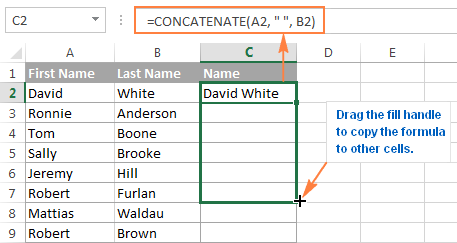
6. Change Text to Lower/Upper/Proper Case

While importing data, we often find names in irregular forms like lower, upper case, or sometimes mixed. Such errors are not easy to eliminate manually. Here’s a fingertip trick to bring back the consistency.

• LOWER(text)
• UPPER(text)
• PROPER(text)

Steps:

• Just type the formula you want to use, suppose “LOWER(“ and select the cell whose case needs to be changed.
• Hit “CTRL+ENTER.”
• The case has been changed & Consistent
• Drag down to do the same for other cells.
• Similarly for UPPER() & PROPER()

7. Parse Data Using Text to Column

Sometimes the received Data has texts filled in one cell, only separated by punctuations. Usually, the addresses are cramped in one cell separated by a comma. To distinguish values in separate cells, we can use “Text to Column.”

Steps:

• Select the Data
• Go to Data> Text to Column
• A dialogue box will appear (Convert Text to Columns Wizard – Step 1 of 3), select Delimited or Fixed Width as per your convenience.
• Delimited is to be selected if the width isn’t fixed, click “NEXT”
• In Delimiters tick the option which separates your text in the cell. Suppose “Norwich Cathedral, Norwich, UK,” here three values are separated by commas. So we will select “Comma” for this example. And, deselect the rest options.
• View the preview & click on “NEXT”
• Select Column Data Format & destination cell address
• Click “FINIS

8. Spell Check

Spelling mistakes are common in text files & PowerPoint. However, MS points out such errors by underlining them with colourful dashes. And, MS Excel doesn’t have such a feature. But you can use it below steps to clean data on excel.

• Select the Data
• Press “F7”
• A dialogue box appears, which shows you the possible wrong word & it’s the possible correct spelling. Click on “Change,” if you agree with the suggestion.
• Check & change till it says “Spell check complete. You’re good to go!”

9. Delete all Formatting

In my job, I used multiple databases to get the data in excel. Every database had it’s own data formatting. When you have all the data in place, here is how you can delete all the formatting in one go:

1. Select the data set
2. Go to Home –> Clear –> Clear Formats

Similarly, you can clear Content, Comments, Hyperlink, or entire data (using Clear All).

10. Use Find & Replace to Clean Data in Excel

A) Changing Cell References:

• Press “CTRL+H” to open “Find and Replace”
• Now in Replace > “Find What” (change the reference range too) “Replace With”
• Suppose Find What: $B to Replace With $C
• Click on “Replace All”
• Similarly finding & replacing using reference range we can clean the Data

B) Find & Change Specific Format:

• Press “CTRL+H”
• Select “Options”
• Now go to “Format” of “Find What.” Here you can specify the format or choose a format from the cell. Suppose you select a format.
• Now it will show you the preview for “Find What.”
• Click on “Format” of “Replace With.” Suppose we go for “Format…”
• Now select format, for example, Number, Alignment, Font, Border, Fill, Protection.
• Suppose we select Color and then select any colour to fill the column header cell.
• Click on Replace All
• Instantly the format has been changed!

C) Removal of Line Breaks:

Suppose we have data where it is separated by line breaks (same cell but different rows). To remove these line breaks, follow the below steps:

• Press “CTRL+H”
• Find and Replace dialogue box will appear, press “CTRL+J”
• Go to the replace with box & type a single space
• Click Replace All
• All rows will be managed in one row within the same cell!

D) Removal of Parenthesis:

• Select the Data
• Press “CTRL+H”
• Type (*) in “Find What” (This will consider all characters within parenthesis)
• Leave the Replace With column empty & click Replace
• Parenthesis characters are removed!