Statistics

What Facebook Advertising Data Can Teach Us About Marketing

Businesses spend money showing their products and services on Facebook every day. But spending more money doesn’t guarantee better results.

To understand this better, let’s look at a Facebook advertising dataset containing information from 1,143 advertisements.

We will look at a few simple questions:

  • Which campaigns performed better?
  • Which age groups were reached?
  • How many people clicked on the ads?
  • How much money was spent?
  • How many people converted?
  • What can businesses learn from this data?

The goal is not to build a complicated mathematical model. Instead, let’s use data to understand what was happening behind the advertisements.
What Information Do We Have?

Each row in the dataset represents an advertisement.

For each ad, we have information such as:

  • The campaign it belonged to
  • The target age group
  • Gender
  • Interest category
  • Number of times the ad was shown
  • Number of clicks
  • Money spent
  • Number of conversions
  • Number of approved conversions

Think of it as a report card for Facebook advertisements.

First, Let’s Look at the Numbers

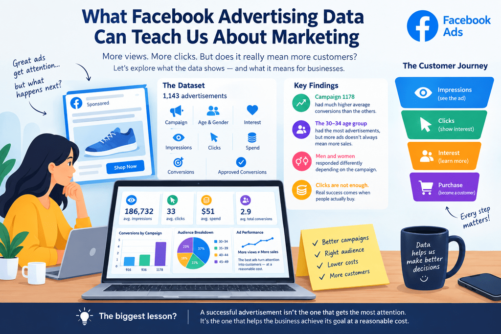
On average, each advertisement was shown about 186,732 times.

However, the average can be misleading because some advertisements were shown millions of times while others were shown much less.

On average, each advertisement received about 33 clicks.

The average advertising spend was about $51.

An advertisement generated around 2.9 total conversions on average, while approved conversions averaged about 0.94.

These numbers tell us something important:

Getting people to see an advertisement is much easier than getting them to take meaningful action.

That is an important lesson for any business running online advertising.

Which Campaign Did Better?

The dataset contains three main campaigns:

  • Campaign 916
  • Campaign 936
  • Campaign 1178

When we compare their average conversions, we see a noticeable difference.

CampaignAverage Total ConversionsAverage Approved Conversions
9161.070.44
9361.160.39
11784.271.40

Campaign 1178 had a much higher average number of conversions per advertisement.

That makes it interesting. But we should be careful. It would be wrong to say:

“Campaign 1178 was definitely better because it caused more sales.”

We don’t have enough information to prove that. Maybe the campaign had a different audience. Maybe it promoted a different product. Maybe it received a different budget. The data tells us that Campaign 1178 had higher conversion numbers in this dataset. It does not tell us exactly why. That’s an important difference.

What About Age?

The advertisements targeted different age groups.

The largest group in the dataset was people aged 30–34.

The other groups were:

  • 35–39
  • 40–44
  • 45–49

There were 426 advertisements targeting people aged 30–34, making it the largest group in the dataset.

But here’s another important lesson.

Having more advertisements aimed at a particular age group doesn’t automatically mean that group is the most profitable.

Imagine a business shows:

1,000 ads to Group A

and

100 ads to Group B.

Group A will probably produce more total clicks simply because it received more exposure.

So marketers should ask:

“How efficiently did each group respond?”

rather than simply:

“Which group produced the most clicks?”

Men vs Women

The dataset contains advertisements targeting both men and women. There are 592 male observations and 551 female observations. This gives us another opportunity to compare advertising performance. But again, we shouldn’t jump to conclusions. Instead of asking:

“Are men better customers than women?”

a better question is:

“How did each audience respond to each campaign?”

A campaign might work well with one audience but poorly with another. This is why businesses often divide their customers into smaller groups instead of treating everyone the same.

Impressions Don’t Mean Sales

One of the biggest lessons from advertising data is that attention is not the same as success. An advertisement can be seen hundreds of thousands of times. People might even click on it. But if nobody buys the product, the business may still lose money. Think about a simple example.

Imagine you spend $100 on an advertisement.

It gets:

100,000 views

2,000 clicks

but only:

1 purchase

At first glance, the advertisement looks impressive.

100,000 views sounds great.

2,000 clicks sound great.

But if the product only generated one purchase, the business needs to ask whether that $100 was worth spending. That’s why businesses need to follow the entire customer journey:

Views → Clicks → Interest → Purchase

Clicks Are Not Enough

A common mistake in digital marketing is focusing too much on clicks. Clicks are useful, but they are only one part of the story. For example:

Ad A

10,000 people see it
500 people click
5 people buy

Ad B

5,000 people see it
200 people click
20 people buy

Ad A gets more clicks.

But Ad B generates more purchases.

So which advertisement should the business investigate further?

The answer cannot be determined from clicks alone.

We need to look at what happens after the click.

What Is CTR?

One simple measurement marketers use is Click-Through Rate, or CTR. It answers a simple question:

“Out of all the people who saw the advertisement, how many clicked it?”

The calculation is:

CTR = Clicks ÷ Impressions × 100

For example, if an advertisement is shown 10,000 times and receives 200 clicks:

CTR = 200 ÷ 10,000 × 100 = 2%

This tells us that 2 out of every 100 impressions resulted in a click.

CTR is useful for understanding how attractive an advertisement is to its audience.

But it still doesn’t tell us whether people bought anything.

What About Advertising Cost?

Businesses also need to know how much they are paying for each result. One simple measurement is Cost Per Click (CPC).

For example:

If a business spends $50 and receives 100 clicks:

CPC = $50 ÷ 100 = $0.50

So each click costs an average of 50 cents. But again, cheap clicks aren’t necessarily good clicks. If those 100 clicks produce zero customers, the business hasn’t achieved much.

The Most Important Number May Be the Final Conversion

For many businesses, the final goal isn’t:

“How many people clicked?”

It’s:

“How many people became customers?”

That’s why conversion data is so important. A simple advertising funnel looks like this:

People see the ad

↓

Some people click

↓

Some people become interested

↓

Some people purchase

At every stage, some people disappear from the funnel. The job of marketing analytics is to understand where that happens.

What Can Businesses Learn From This?

This dataset gives us several useful lessons.

1. More views don’t automatically mean more sales

A popular advertisement can still perform poorly if people don’t take action.

2. More clicks don’t automatically mean more customers

Clicks are only one step in the buying process.

3. Different campaigns can perform very differently

The campaigns in this dataset show clear differences in average conversion numbers.

4. Different audiences can respond differently

Age, gender, and interests can influence how people respond to advertisements.

5. Businesses should look at costs

Getting customers is important, but businesses also need to consider how much they spent to get them.

One Important Warning About Data

There is one thing we should always remember when analyzing marketing data:

Data can show us what happened, but it doesn’t always tell us why it happened.

For example, Campaign 1178 had higher average conversions in this dataset. But we don’t know whether that happened because of:

  • Better advertising
  • Better targeting
  • A better product
  • A larger budget
  • A different audience
  • Better timing
  • Or something else

To answer those questions properly, we would need more information. This is why good data analysis should avoid making claims that the data cannot support.

Final Thoughts

Facebook advertising produces a huge amount of information. But businesses don’t need to look at every number at once. Start with a few simple questions:

How many people saw the ad?

How many clicked?

How much did we spend?

How many people converted?

How much did each customer cost us?

Once we understand these numbers, we can start asking deeper questions about campaigns and audiences. The biggest lesson from this analysis is simple:

A successful advertisement isn’t necessarily the one that gets the most attention. It’s the one that helps the business achieve its goal at a reasonable cost.

That is where data analytics becomes useful. Instead of guessing which advertisement is working, businesses can use their data to understand what happened and make better-informed marketing decisions.

Multivariate Generalized Linear Mixed Models (MGLMMs) in R

Multivariate Generalized Linear Mixed Models (MGLMMs) are an advanced class of statistical models designed to analyze multiple correlated response variables that follow non-Gaussian distributions and arise from hierarchical or clustered data structures. These models extend Generalized Linear Mixed Models (GLMMs) by simultaneously modeling several outcomes while accounting for within-subject or within-cluster correlations.

MGLMMs are especially useful in domains such as biostatistics, psychometrics, and ecology, where repeated measurements, longitudinal data, or nested sampling designs are common. By incorporating both fixed effects (systematic influences) and random effects (subject-specific variability), MGLMMs provide a flexible and robust framework for inference.

Advantages of MGLMMs:

  • Handle correlated outcomes.
  • Accommodate non-normal response distributions (e.g., binary, count).
  • Incorporate hierarchical structures via random effects.
  • Joint modeling improves efficiency and consistency of parameter estimates.

Model Specification

Let Yij=(Yij1,Yij2,…,Yijp)TY_{ij} = (Y_{ij1}, Y_{ij2}, \ldots, Y_{ijp})^T denote a vector of pp response variables for subject ii at occasion jj. The MGLMM can be written as:

gk(E[Yijk∣bi])=XijkTβk+ZijkTbik,k=1,…,pg_k(\mathbb{E}[Y_{ijk} | b_i]) = \mathbf{X}_{ijk}^T\boldsymbol{\beta}_k + \mathbf{Z}_{ijk}^T\mathbf{b}_{ik}, \quad k = 1, \ldots, p

Where:

  • gk(⋅)g_k(\cdot): Link function for the kk-th outcome (e.g., logit, log).
  • Xijk\mathbf{X}_{ijk}: Covariates associated with fixed effects βk\boldsymbol{\beta}_k.
  • Zijk\mathbf{Z}_{ijk}: Covariates associated with random effects bik\mathbf{b}_{ik}.
  • bi=(bi1,…,bip)∼N(0,D)\mathbf{b}_i = (\mathbf{b}_{i1}, \ldots, \mathbf{b}_{ip}) \sim \mathcal{N}(0, \mathbf{D}): Multivariate normal random effects capturing within-subject correlation.

Assumptions:

  • Responses are conditionally independent given the random effects.
  • Var(Yijk∣bi)=ϕkVk(μijk)\text{Var}(Y_{ijk} | b_i) = \phi_k V_k(\mu_{ijk}), where ϕk\phi_k is a dispersion parameter.
  • Cross-covariance between random effects models indicates dependencies among outcomes.

Multivariate Generalized Linear Mixed Models (MGLMMs) in R

Multivariate Generalized Linear Mixed Models (MGLMMs) in R

Download:

Implementation in R

Several R packages support MGLMMs. Below is a step-by-step guide using glmmTMB, MCMCglmm, and brms for Bayesian approaches.

Data Preparation

library(glmmTMB)
data(Salamanders)
str(Salamanders) # Binary response: Presence/absence across sites and species

Fitting a Bivariate Model (e.g., Count and Binary Responses)

# Example using glmmTMB for two outcomes with random effects
fit <- glmmTMB(cbind(count, binary) ~ spp * mined + (1 | site),
               data = mydata,
               family = list(poisson(), binomial()))
summary(fit)

Using MCMCglmm for Multivariate Bayesian GLMMs

library(MCMCglmm)
prior <- list(R = list(V = diag(2), nu = 0.002),
              G = list(G1 = list(V = diag(2), nu = 0.002)))

fit <- MCMCglmm(cbind(trait1, trait2) ~ trait - 1 + trait:(fixed_effects),
                random = ~ us(trait):ID,
                rcov = ~ us(trait):units,
                family = c("categorical", "poisson"),
                data = mydata,
                prior = prior,
                nitt = 13000, burnin = 3000, thin = 10)
summary(fit)

Model Diagnostics

  • Check convergence (trace plots, effective sample size)
  • Use DHARMa for residual diagnostics with glmmTMB
  • Posterior predictive checks with bayesplot or pp_check in brms

Case Study: Predicting Educational Outcomes

Dataset: Simulated dataset with students (nested in schools), outcomes: math score (Gaussian) and pass/fail (binary).

Research Question:

How do student-level and school-level predictors influence academic performance and passing probability?

Modeling:

fit <- glmmTMB(cbind(math_score, passed) ~ gender + SES + (1 | school_id),
               data = edu_data,
               family = list(gaussian(), binomial()))
summary(fit)

Interpretation:

  • Fixed effects show the average association of covariates with each outcome.
  • Random effects estimate school-specific deviations.
  • Correlation structure shows how math scores and passing status co-vary within schools.

Visualization:

library(ggplot2)
# Predicted vs Observed
edu_data$pred_math <- predict(fit)[,1]
ggplot(edu_data, aes(x = pred_math, y = math_score)) +
  geom_point() + geom_smooth()

Challenges and Solutions

Common Issues:

  • Convergence problems: Simplify model, check starting values, use penalized likelihood.
  • Non-identifiability: Avoid overparameterization; regularize random effects.
  • Model misspecification: Perform residual diagnostics; compare with nested models.

Expert Tips:

  • Always examine the random effects structure.
  • Use informative priors in Bayesian settings.
  • Scale predictors to improve convergence.

Extensions and Alternatives

  • GEEs: Useful for marginal models but less flexible for hierarchical data.
  • Bayesian hierarchical models: Rich inference, handles uncertainty better.
  • Joint modeling: For longitudinal and survival data.

MGLMMs are most appropriate when multiple correlated outcomes are influenced by shared covariates and random effects structures.

References

  1. McCulloch, C. E., Searle, S. R., & Neuhaus, J. M. (2008). Generalized, Linear, and Mixed Models. Wiley.
  2. Brooks, M. E., Kristensen, K., van Benthem, K. J., et al. (2017). glmmTMB balances speed and flexibility among packages for zero-inflated generalized linear mixed modeling. The R Journal.
  3. Hadfield, J. D. (2010). MCMC Methods for Multi-Response Generalized Linear Mixed Models: The MCMCglmm R Package. Journal of Statistical Software.
  4. Gelman, A., et al. (2013). Bayesian Data Analysis. CRC Press.
  5. Bolker, B. M., et al. (2009). Generalized linear mixed models: a practical guide for ecology and evolution. Trends in Ecology & Evolution.

For advanced users, packages such as brms and rstanarm offer flexible Bayesian interfaces for MGLMMs, enabling greater control over model specification and inference.

Download (PDF)

Read More: Applied Multivariate Statistics with R

Mastering Advanced Statistics Using R

Statistics is the backbone of data-driven decision-making, and R has become the go-to tool for statisticians and data analysts worldwide. With its rich ecosystem of libraries and intuitive syntax, R simplifies complex statistical analysis and empowers users to extract actionable insights from data. This blog will walk you through the fundamentals and advanced features of R for statistics, ensuring you unlock the full potential of this powerful programming language.

Why Use R for Advanced Statistics?

R excels in statistical computing for several reasons:

  1. Specialized Libraries: Packages like dplyr, ggplot2, caret, and MASS provide functionalities tailored to various statistical needs.
  2. Data Visualization: R offers state-of-the-art visualization tools that make your statistical findings easy to interpret and present.
  3. Community Support: A vibrant community ensures frequent updates, new packages, and a wealth of learning resources.
  4. Flexibility and Integration: R integrates seamlessly with Python, SQL, and big data tools like Hadoop and Spark.

    Download PDF

Key Features for Advanced Statistical Analysis

1. Linear and Non-linear Modeling

  • Linear Regression: The lm() function in R is a powerful tool for predicting relationships between variables.
  • Non-linear Models: R handles complex relationships using functions like nls() and packages like nlme.

Example:

model <- lm(y ~ x1 + x2, data = dataset)
summary(model)

2. Multivariate Analysis

Techniques like Principal Component Analysis (PCA) and Cluster Analysis can be implemented easily using libraries like stats and FactoMineR.

  • PCA: Dimensionality reduction to simplify datasets.
  • Cluster Analysis: Grouping similar observations for pattern recognition.

3. Time-Series Analysis

R’s forecast and tsibble packages are tailored for analyzing and predicting trends over time.
Example:

library(forecast)
fit <- auto.arima(time_series_data)
forecast(fit, h = 10)

4. Bayesian Statistics

R integrates Bayesian methods through packages like rstan and bayesplot. These tools allow you to perform probabilistic modeling and inference.

5. Machine Learning Integration

With packages like caret and mlr, you can blend statistical analysis with machine learning techniques, from decision trees to ensemble methods.

How to Get Started with R for Advanced Statistics?

Step 1: Install Essential Libraries

Start by installing foundational libraries:

install.packages(c("dplyr", "ggplot2", "caret", "MASS"))

Step 2: Understand Your Data

Explore your dataset with summary statistics and visualizations:

summary(dataset)
plot(dataset$x, dataset$y)

Step 3: Apply Advanced Methods

Dive into specific statistical techniques that match your project needs, from regression to hypothesis testing.

Tips for Mastering R for Advanced Statistics

  1. Leverage Online Resources: Use platforms like CRAN, Stack Overflow, and R-bloggers for learning.
  2. Practice Regularly: Build projects, analyze real-world datasets, and replicate case studies to sharpen your skills.
  3. Focus on Visualization: Master ggplot2 to create compelling visual narratives for your analyses.

Conclusion

Advanced statistics using R opens up endless possibilities for data exploration, modeling, and prediction. Whether you’re analyzing large datasets or diving deep into Bayesian methods, R equips you with the tools needed for success. Start today, and transform your data into impactful insights.

Download: Applied Statistics: Theory and Problem Solutions with R

R Cheat Sheet For Everyone

R is a powerful programming language used for data analysis and statistical computing. Here is a quick reference guide to get you started with R programming.

R Cheat Sheet For Everyone

Basic Syntax:

  • Comments start with the “#” symbol
  • Assignment operator is “<-“
  • Function calls use parentheses, e.g. mean(x)
  • “print()” function can be used to display results
  • Use “?” before a function to get help, e.g. ?mean

Data Types:

  • Numeric: numbers with decimal places, e.g. 3.14
  • Integer: whole numbers, e.g. 5
  • Character: text, e.g. “hello”
  • Factor: categorical data, e.g. “male” or “female”
  • Logical: binary values, either TRUE or FALSE

Vectors:

  • A vector is a collection of values with the same data type
  • Creation of vectors using c(), e.g. c(1,2,3)
  • Use “[]” to access elements of a vector, e.g. x[2]
  • Use “length()” to get the number of elements in a vector

Matrices:

  • A matrix is a 2-dimensional vector with rows and columns
  • Creation of matrices using matrix(), e.g. matrix(1:9, ncol=3)
  • Use “[row, col]” to access elements of a matrix, e.g. m[2,3]
  • Use “dim()” to get the dimensions of a matrix

DataFrames:

  • A data frame is a 2-dimensional data structure with rows and columns
  • Creation of data frames using data.frame(), e.g. data.frame(x=1:5, y=6:10)
  • Use “$” to access columns of a data frame, e.g. df$x
  • Use “nrow()” and “ncol()” to get the number of rows and columns

Reading Data:

  • Use read.csv() to read csv files, e.g. read.csv(“data.csv”)
  • Use read.table() to read other types of files, e.g. read.table(“data.txt”, sep=”\t”)

Data Manipulation:

  • Use “head()” and “tail()” to view the first and last few rows of a data frame
  • Use “subset()” to extract a subset of a data frame based on conditions, e.g. subset(df, x > 3)
  • Use “merge()” to combine two data frames based on common columns

Plotting:

  • Use “plot()” to create basic plots, e.g. plot(x, y)
  • Use “hist()” to create histograms, e.g. hist(x)
  • Use “boxplot()” to create box plots, e.g. boxplot(x)
  • Use “barplot()” to create bar plots, e.g. barplot(x)

Statistics:

  • Use “mean()” to calculate the mean of a vector, e.g. mean(x)
  • Use “median()” to calculate the median of a vector, e.g. median(x)
  • Use “sd()” to calculate the standard deviation of a vector, e.g. sd(x)
  • Use “summary()” to get a summary of a data frame, e.g. summary(df)

Most Important Algorithms That You Should Know

Algorithms are used by all of us all the time with or without our direct knowledge. They have applications in many different disciplines, from math and physics to, of course, computing. These are the most important algorithms that you should know.

1. Boolean (binary) algebra

You might be familiar with the term Boolean from mathematics, logic, and computer coding. It was created by  George Boole in 1847 work An Investigation of the Laws of Thought. Boolean algebra is a branch of algebra in which a variable can only ever be true or false (usually binary 1 or 0). This algorithm is widely recognized as the foundation of modern computer coding. It is still in use today, especially in computer circuitry.

Logic gate and Boolean algebra (updated) - PLACIDE'S PERSONAL BLOG
Most Important Algorithms That You Should Know: Logic gates and Boolean algebra

2. Fast Fourier Transform

This algorithm was created by Carl Gauss, Joseph Fourier, James Cooley, and John Tukey in 1802, 1822 and 1965. It is used to break down a signal into the frequencies that compose it – much like a musical chord can be expressed in frequencies, or pitches, of each note therein. “FFT relies on a divide-and-conquer strategy to reduce an ostensibly O(N2) chore to an O(N log N) frolic.

Login to add a new term or to edit a term you have once submitted Email  address Password Encyclopedia Home Ultrasonic Testing (UT) Fast Fourier  Transformation Abbreviation: FFT, Related Entries: bandwidth, Exhibitors  Keywords: EKOSCAN.. • Articles ...
Most Important Algorithms That You Should Know: FFT – Fast Fourier Transformation

3. Google’s ranking algorithm

PageRank is, arguably, the most used algorithm in the world today. It is, of course, the foundation of the ranking of pages on Google’s search engine. It was created by Larry Page (mainly) and Sergey Brin in 1996.  It is not the only algorithm that Google uses nowadays to order pages on its search result, but it is the oldest and best known of them.

The PageRank algorithm is given by the following formula:

PR(A) = (1-d) + d (PR(T1)/C(T1) + … + PR(Tn)/C(Tn))

where:

  • PR(A) is the PageRank of page A,
  • PR(Ti) is the PageRank of pages Ti which links to page A,
  • C(Ti) is the number of outbound links on page Ti and;
  • d is a damping factor that can be set between 0 and 1.
Google confirms mid-December search ranking algorithm updates
Most Important Algorithms That You Should Know

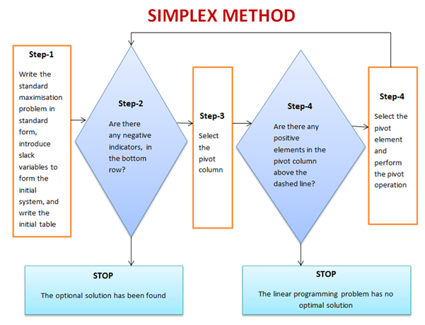
4. The simplex method for linear programming

This is one of the most successful algorithms of all time despite the fact that most real-world problems are rarely linear in nature. It was created by George Dantzig in 1947. It was widely used in the world of industry or any other situation where economic survival rests on the ability to maximize efficiency within a budget and/or other constraints.

It works by using a systematic strategy to generate and validate candidate vertex solutions within a linear program. At each iteration, the algorithm chooses the variable that makes the biggest modification towards the minimum-cost solution. That variable then replaces one of its covariables, which is most drastically limiting it, thereby shifting the simplex method to another part of the solution set and toward the final solution. 

Linear Programming Problems, Linear Programming Simplex Method
Most Important Algorithms That You Should Know

5. Kalman Filter

Kalman Filtering, aka linear quadratic estimation (LQE), helps you make an educated guess about what a system will likely do next, within reason, of course. Kalman filters are great for situations where systems are constantly changing.  Created by Rudolf E. Kálmán in 1958-1961  is a general and powerful tool for combining information in the presence of uncertainty.

Kalman filter algorithm. | Download Scientific Diagram
Most Important Algorithms That You Should Know: Kalman Filter algorithm

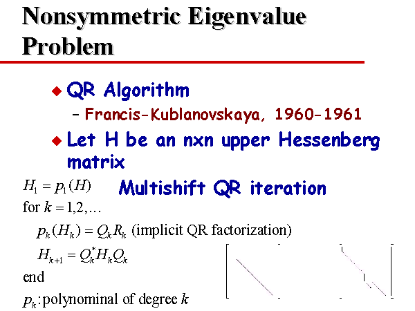
6. QR algorithms for computing eigenvalues

 It was created in the late 1950s by John G. F. Francis and by Vera N. Kublanovskaya independently. The QR algorithm, aka eigenvalue algorithm, greatly simplifies the calculations of eigenvalues it is important in numerical linear algebra. In addition to enabling the swift calculation of eigenvalues, it also aids in the processing of eigenvectors in a given matrix. Its basic function is to perform QR decomposition, write a matrix as a product of an orthogonal matrix and an upper triangular matrix, multiply the factors in the reverse order and iterate.

Nonsymmetric Eigenvalue Problem
Most Important Algorithms That You Should Know: QR algorithms for computing eigenvalues

7. JPEG and other data compression algorithms

It was created in 1992 by the Joint Photographic Experts Group, IBM, Mitsubishi Electric, AT&T, Canon Inc., and ITU-T Study Group 16. It is difficult to single out one particular data compression algorithm as its value or importance depends on the files’ applications. Data compression algorithms, like JPEG, MP3, zip, or MPEG-2, are widely used the world over. Most have become the de facto standard for their particular application. They have made computer systems cheaper and more efficient over time.

JPEG compression algorithm.  
Most Important Algorithms That You Should Know: JPEG compression algorithm.  

8. Quicksort algorithm

Created by Tony Hoare of Elliott Brothers, Limited, London in 1962. It provided a means of quickly and efficiently sorting lists alphabetically and numerically. Quicksort algorithm used a recursive strategy to “divide and conquer” to rapidly reach a solution. It would prove to be two to three times quicker than its main competitors’ merge sort and heapsort. It works by choosing one element to be the “pivot”. All others are then sorted into “bigger” and “smaller” piles of elements relative to the pivot. This process is then repeated in each pile. 

Quicksort Algorithm - InterviewBit
Most Important Algorithms That You Should Know: Quicksort algorithm

Best Statistical Analysis Software

Statistical software is a specialized computer program which helps you to collect, organize, analyze, interpret and statistically design data. There are two main statistical techniques which help in statistical data analysis: descriptive statistics and inferential statistics.

Descriptive statistics organize data from a sample using indexes. Inferential statistics draw a conclusion from data that is a random variant. Statistics are crucial for organizations. They provide factual data which is critical in detecting trends in the marketplace so that businesses can compare their performance against their competitors. These are the best statistical analysis software:

1. SPSS (IBM)

SPSS, (Statistical Package for the Social Sciences) is perhaps the most widely used statistical software package in human behaviour research. SPSS offers the ability to easily compile descriptive statistics, parametric and non-parametric analyses, as well as graphical depictions of results through the graphical user interface (GUI). It also includes the option to create scripts to automate analysis or to carry out more advanced statistical processing.

2.RStudio

The primary mission of RStudio is to build a sustainable open-source business that creates software for data science and statistical computing. You may have already heard of some of our work, such as the RStudio IDE, Rmark down, shiny, and many packages in the tidy verse. Our open-source projects are supported by our commercial products that help teams of R users work together effectively, share computing resources, and publish their results to decision-makers within the organization. 

3. Stata

Stata: Software for Statistics and Data Science

Stata puts hundreds of statistical tools at your fingertips. For data management, statistical analysis, and publication-quality graphics, Stata has you covered.

4. OriginPro

Origin is a user-friendly and easy-to-learn software application that provides data analysis and publication-quality graphing capabilities tailored to the needs of scientists and engineers. OriginPro offers extended analysis tools for Peak Fitting, Surface Fitting, Statistics, Signal Processing and Image Handling. Users can customize operations such as importing, graphing and analysis, all from the GUI. Graphs, analysis results and reports update automatically when data or parameters change. 

5. Microsoft Excel

microsoft excel

While not a cutting-edge solution for statistical analysis, MS Excel does offer a wide variety of tools for data visualization and simple statistics. It’s simple to generate summary metrics and customizable graphics and figures, making it a useful tool for many who want to see the basics of their data. As many individuals and companies both own and know how to use Excel, it also makes it an accessible option for those looking to get started with statistics.

Have you read this: Data Science: Free Online Courses For 2020

6. SAS Base

SAS BASE

SAS Base is a programming language software that provides a web-based programming interface; ready-to-use programs for data manipulation, information storage and retrieval, descriptive statistics and reporting; a centralized metadata repository; and a macro facility that reduces programming time and maintenance headaches.

7. MATLAB

Matlab

MatLab is an analytical platform and programming language that is widely used by engineers and scientists. As with R, the learning path is steep, and you will be required to create your own code at some point. A plentiful amount of toolboxes are also available to help answer your research questions (such as EEGLab for analysing EEG data). While MatLab can be difficult to use for novices, it offers a massive amount of flexibility in terms of what you want to do as long as you can code it.

8. Analyse-it

Analyse-it

Analyse-it is a statistical analysis software that includes hypothesis testing, model fitting, ANOVA, PCA, statistical process control (SPC) and quality improvement, and analytical and diagnostic method validation for laboratories to meet regulatory compliance.

9. GraphPad Prism

GraphPad Prism

GraphPad Prism is premium software primarily used within statistics related to biology but offers a range of capabilities that can be used across various fields. Similar to SPSS, scripting options are available to automate analyses, or carry out more complex statistical calculations, but the majority of the work can be completed through the GUI.

10. Minitab

Minitab

The Minitab software offers a range of both basic and fairly advanced statistical tools for data analysis. Similar to GraphPad Prism, commands can be executed through both the GUI and scripted commands, making it accessible to novices as well as users looking to carry out more complex analyses.