Understanding Correlation Coefficient and Correlation Test in R: In the world of data science and statistics, understanding relationships between variables is crucial. One common way to measure the strength and direction of such relationships is through correlation. The correlation coefficient quantifies how strongly two variables are related, while a correlation test helps determine whether the observed correlation is statistically significant. In this guide, we’ll dive deep into these concepts and learn how to implement them in R, one of the most widely used programming languages for statistical computing.
What is a Correlation Coefficient?
The correlation coefficient is a numerical measure of the strength and direction of a linear relationship between two variables. The most commonly used correlation measure is the Pearson correlation coefficient, denoted as r. Its value ranges between -1 and +1:
- r = 1: A perfect positive correlation, meaning as one variable increases, the other also increases in a perfectly linear manner.
- r = -1: A perfect negative correlation, meaning as one variable increases, the other decreases in a perfectly linear manner.
- r = 0: No correlation, meaning there is no linear relationship between the two variables.
In practice, correlation coefficients rarely hit the extremes of +1 or -1. Values closer to 0 indicate weak correlations, while values closer to ±1 suggest stronger correlations.
Types of Correlation Coefficients
- Pearson Correlation: Measures linear relationships between variables.
- Spearman’s Rank Correlation: Used for ordinal data or when the data does not meet the assumptions of normality, Spearman’s correlation evaluates monotonic relationships.
- Kendall’s Tau: Another non-parametric correlation measure used when data do not meet the assumptions of Pearson’s correlation.
How to Calculate Correlation in R
R provides an easy and efficient way to calculate correlation coefficients between variables. Here’s an example of how to do it:
# Create two variables
x <- c(10, 20, 30, 40, 50)
y <- c(15, 25, 35, 45, 60)

# Calculate Pearson correlation
cor(x, y)
In this case, cor(x, y) will return the Pearson correlation coefficient between the two variables x and y. By default, the cor() function in R calculates the Pearson correlation, but you can easily switch to Spearman or Kendall by specifying the method:
# Spearman correlation
cor(x, y, method = "spearman")

# Kendall correlation
cor(x, y, method = "kendall")
Interpreting the Correlation Coefficient
- r > 0: Positive correlation (as one variable increases, the other tends to increase).
- r < 0: Negative correlation (as one variable increases, the other tends to decrease).
- r = 0: No correlation.
In real-world data, a correlation of 0.7 or higher is often considered a strong correlation, while anything between 0.3 and 0.7 indicates a moderate correlation. Values below 0.3 suggest weak correlation.
Correlation Test in R
While the correlation coefficient gives you a measure of association, it’s also important to assess whether the observed correlation is statistically significant. This is where a correlation test comes in. It provides a p-value to determine if the correlation you’ve observed could have arisen by random chance.
You can perform a correlation test using the cor.test() function in R. This function returns a p-value, confidence intervals, and the correlation coefficient.
Here’s how to use it:
# Correlation test
cor.test(x, y)
The output will give you:
- t: The t-statistic used to assess the significance of the correlation.
- p-value: A p-value less than 0.05 (typically) indicates that the correlation is statistically significant.
- Confidence Interval: The range within which the true correlation is likely to fall.
Example of Correlation Test
Let’s perform a real example with random data:
# Generating random data
set.seed(123)
x <- rnorm(100)  # 100 random numbers from a normal distribution
y <- x + rnorm(100)

# Correlation test
cor.test(x, y)
The output will give us the Pearson correlation coefficient and the p-value. If the p-value is below 0.05, we reject the null hypothesis, concluding that there is a significant correlation between x and y.
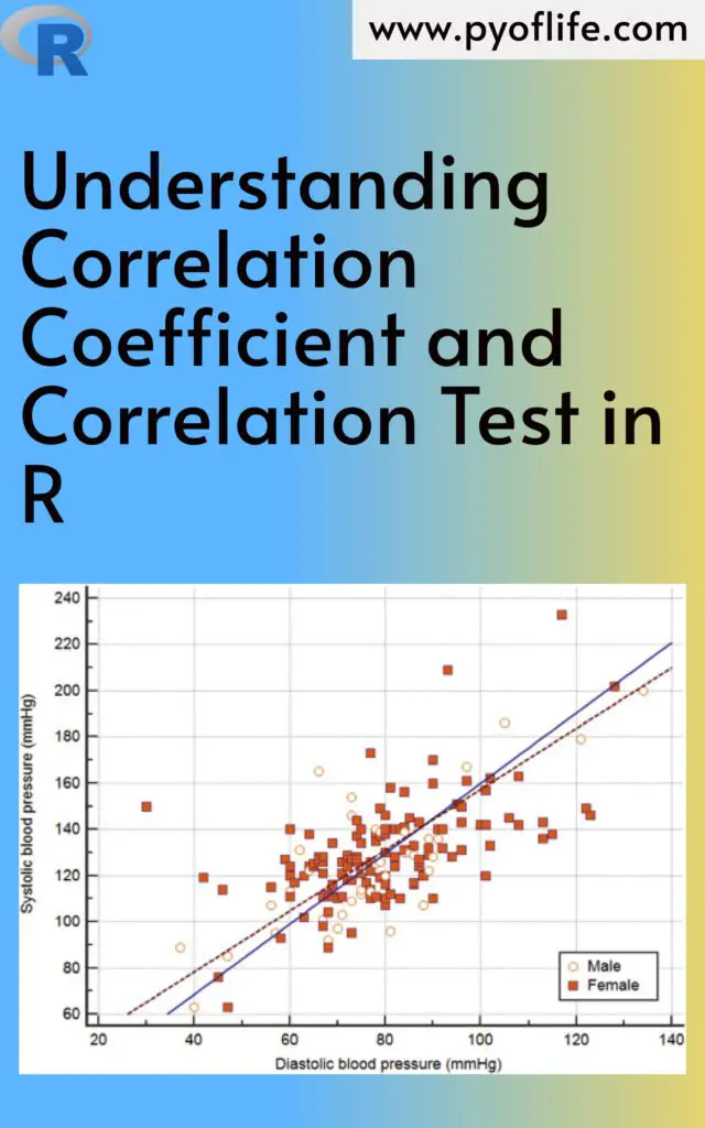
Visualizing Correlation
Visualizing correlations can give additional insight into relationships between variables. A common way to visualize correlation is through a scatter plot with a fitted regression line. You can use R’s ggplot2 package for this:
library(ggplot2)

# Creating a scatter plot with regression line
ggplot(data.frame(x, y), aes(x = x, y = y)) +
  geom_point() +
  geom_smooth(method = "lm", col = "blue") +
  theme_minimal() +
  labs(title = "Scatter Plot with Correlation", x = "X Variable", y = "Y Variable")
This plot will display the relationship between x and y and provide visual confirmation of whether the variables appear to be correlated.
Limitations of Correlation
It’s important to note that correlation doesn’t imply causation. Even if two variables are strongly correlated, it doesn’t mean one causes the other. There could be other factors at play, or the correlation could be spurious.
Additionally, the Pearson correlation measures only linear relationships. If your data have a non-linear relationship, the correlation coefficient may not accurately capture the strength of the relationship. In such cases, consider using Spearman’s or Kendall’s correlation.
Conclusion
Understanding the correlation coefficient and conducting correlation tests are essential skills for anyone working with data. They help you uncover relationships between variables and determine the significance of those relationships. With R, calculating and testing correlations is straightforward, whether you’re working with linear data or need to rely on non-parametric methods.
By mastering these techniques, you can gain deeper insights into your data, uncover meaningful patterns, and drive more informed decision-making in your analyses.
By using the cor() and cor.test() functions in R, along with visualization tools likeggplot2, you’re well-equipped to analyze and interpret correlations in any dataset. Whether you’re a beginner or an experienced data scientist, these methods form the foundation of many statistical analyses.
Download: Linear Regression Using R: An Introduction to Data Modeling