PYOFLIFE

Introduction to Basic Statistics with R: Statistics is a branch of mathematics that deals with the collection, analysis, interpretation, presentation, and organization of data. It has become an essential tool in many fields, including science, engineering, medicine, business, and economics. In this article, we will introduce you to the basic statistics concepts and their implementation in R, a popular statistical programming language.

Step 1: Installing R and RStudio The first step in using R for statistical analysis is to install R and RStudio. R is a programming language for statistical computing and graphics, while RStudio is an integrated development environment (IDE) for R.

Step 2: Getting Started with R After installing R and RStudio, you can launch RStudio and start using R. The RStudio interface has several panes, including the console, editor, and workspace. The console is where you can enter commands and see the results. The editor is where you can write and save R code, while the workspace displays the objects and data structures in your environment.

Step 3: Basic Statistical Concepts Before we start using R, let’s review some basic statistical concepts. The following are some of the most common statistical terms:

• Population: A population is a group of individuals or objects that we want to study.
• Sample: A sample is a subset of the population that we collect data from.
• Variable: A variable is a characteristic or attribute that we measure.
• Data: Data is the information that we collect from the variables.
• Descriptive Statistics: Descriptive statistics are methods that summarize and describe the characteristics of the data, such as measures of central tendency, measures of dispersion, and graphs.
• Inferential Statistics: Inferential statistics are methods that use sample data to make inferences or predictions about the population.

Step 4: Data Import and Manipulation To start analyzing data in R, you need to import it into the R environment. R can read data from various file formats, such as CSV, Excel, and text files. Once you have imported your data, you can manipulate it using various functions and operators, such as subsetting, merging, and filtering.

Step 5: Descriptive Statistics in R R provides several functions for calculating descriptive statistics. The following are some of the most common descriptive statistics functions in R:

• mean(): calculates the arithmetic mean of a vector or a matrix
• median(): calculates the median of a vector or a matrix
• sd(): calculates the standard deviation of a vector or a matrix
• var(): calculates the variance of a vector or a matrix
• summary(): provides a summary of the data, including the minimum, maximum, quartiles, mean, and median.

Step 6: Inferential Statistics in R R provides several functions for performing inferential statistics. The following are some of the most common inferential statistics functions in R:

• t.test(): performs a t-test for two samples or one sample
• cor(): calculates the correlation coefficient between two variables
• lm(): performs linear regression analysis
• chisq.test(): performs a chi-squared test for independence
• anova(): performs analysis of variance (ANOVA)

Step 7: Data Visualization in R Data visualization is an essential part of statistical analysis. R provides several packages for creating various types of graphs, such as bar charts, scatter plots, line charts, and histograms. The following are some of the most common data visualization packages in R:

• ggplot2: a package for creating elegant and customizable graphs
• lattice: a package for creating complex graphs with multiple panels
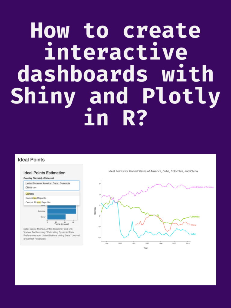
• plotly: a package for creating interactive graphs
• ggvis: a package for creating interactive and customizable graphs

Geovisualization is the process of displaying geospatial data in a visual form that helps people better understand and interpret data. R is a popular programming language for data analysis and visualization, and it has several packages that make it easy to create interactive geo visualizations. In this article, we will explore some of the R packages that can be used to create interactive geo visualizations.

1. ggplot2

ggplot2 is a popular package for creating static visualizations in R. However, it can also be used to create interactive geo visualizations. The ggplot2 package provides the geom_sf() function, which can be used to plot spatial data. The sf package is used to read spatial data, and the dplyr package can be used to manipulate the data. The plotly package can be used to create interactive plots from ggplot2 objects.

Here is an example of creating an interactive plot using ggplot2 and plotly:

library(sf)
library(ggplot2)
library(dplyr)
library(plotly)

# Read the spatial data
data <- st_read("path/to/data.shp")

# Group the data by a variable
data_grouped <- data %>% group_by(variable)

# Create the plot
plot <- ggplot() + 
  geom_sf(data = data_grouped, aes(fill = variable)) + 
  scale_fill_viridis_c() +
  theme_void()

# Create the interactive plot
ggplotly(plot)

2. Leaflet

Leaflet is a popular JavaScript library for creating interactive maps. The leaflet package provides an interface to the Leaflet library, which can be used to create interactive maps in R. The package provides several functions for creating interactive maps, including addTiles(), addMarkers(), addPolygons(), and addPopups().

Here is an example of creating an interactive map using the leaflet package:

library(leaflet)
library(sf)

# Read the spatial data
data <- st_read("path/to/data.shp")

# Create the map
map <- leaflet(data) %>% addTiles() %>%
  addPolygons(fillColor = ~pal(variable)(variable),
              weight = 2,
              opacity = 1,
              color = "white",
              fillOpacity = 0.7) %>%
  addLegend(pal = pal, values = ~variable,
            title = "Variable",
            opacity = 0.7)

# Define the color palette
pal <- colorNumeric(palette = "YlOrRd", domain = data$variable)

# Display the map
map

3. tmap

tmap is a package for creating thematic maps in R. It provides several functions for creating interactive maps, including tm_shape(), tm_fill(), tm_basemap(), and tm_layout(). The package also provides several color palettes for visualizing data.

Here is an example of creating an interactive map using the tmap package:

library(tmap)
library(sf)

# Read the spatial data
data <- st_read("path/to/data.shp")

# Create the map
map <- tm_shape(data) + 
  tm_fill("variable", palette = "Blues", style = "quantile") + 
  tm_basemap("Stamen.TonerLite") + 
  tm_layout(title = "Interactive Map")

# Display the map
tmap_leaflet(map)

How to create interactive dashboards with Shiny and Plotly in R? Creating interactive dashboards is an important task in data analysis and visualization. Dashboards provide a way to visualize data and communicate insights to stakeholders. In this article, we will explore how to create interactive dashboards using Shiny and Plotly in R.

Shiny is a web application framework for R that allows users to create interactive web applications using R. Plotly is a powerful data visualization library that can create interactive visualizations for the web. Together, Shiny and Plotly provide a powerful toolset for creating interactive dashboards.

Setup

Before we start creating our dashboard, we need to install the necessary packages. We will be using the following packages:

install.packages("shiny")
install.packages("plotly")

Once we have installed these packages, we can start building our dashboard.

Building the dashboard

To start building our dashboard, we need to create a new Shiny application. We can do this by running the following command in R:

library(shiny)
shinyApp(ui = ui, server = server)

This will create a new Shiny application with a default user interface (UI) and server function (server).

Adding UI components

Next, we need to add UI components to our dashboard. These components will define the layout and appearance of our dashboard. We will be using the fluidPage function from Shiny to create a responsive UI. The fluidPage function will automatically adjust the layout of the dashboard based on the size of the user’s screen.

ui <- fluidPage(
  # Add UI components here
)

Next, we will add a title to our dashboard using the titlePanel function. We will also add a sidebar with input controls using the sidebarLayout and sidebarPanel functions.

ui <- fluidPage(
  titlePanel("My Dashboard"),
  sidebarLayout(
    sidebarPanel(
      # Add input controls here
    ),
    # Add output components here
  )
)

We can add various input controls to our sidebar using functions such as sliderInput, textInput, checkboxInput, and selectInput. These input controls will allow users to interact with our dashboard and filter or adjust the data displayed.

Adding server logic

Next, we need to add server logic to our dashboard. The server function will define how the dashboard reacts to user input and how it updates the visualizations.

server <- function(input, output) {
  # Add server logic here
}

We can use the renderPlotly function from Plotly to create interactive visualizations in our dashboard. This function takes a plotly object as input and creates an interactive visualization based on the user’s input.

server <- function(input, output) {
  output$plot <- renderPlotly({
    # Create interactive visualization here
  })
}

We can also use the reactive function from Shiny to create reactive expressions that update based on user input. These expressions can be used to filter data, adjust the parameters of visualizations, or perform calculations.

server <- function(input, output) {
  filtered_data <- reactive({
    # Filter data based on user input
  })
  
  output$plot <- renderPlotly({
    # Create interactive visualization based on filtered data
  })
}

Adding interactive visualizations

Finally, we can add interactive visualizations to our dashboard using the plot_ly function from Plotly. This function allows us to create a wide range of interactive visualizations, including scatterplots, bar charts, heatmaps, and more.

server <- function(input, output) {
  filtered_data <- reactive({

Download(PDF)

Econometrics is a branch of economics that uses statistical and mathematical methods to analyze economic data. It is an important tool for economists and policymakers to make informed decisions about economic policies and forecast economic outcomes. R is a programming language widely used in econometrics to analyze, visualize, and interpret data. In this article, we will provide an introduction to econometrics with R. We will discuss the basic concepts of econometrics and how R can be used to apply these concepts.

What is Econometrics?

Econometrics is the application of statistical methods to economic data to test economic theories and forecast economic outcomes. It is used to estimate the relationships between economic variables, such as price and quantity, income and expenditure, and interest rates and investment. Econometrics uses statistical models to describe the relationships between these variables and to make predictions about future economic behavior.

Econometrics involves three steps:

1. Specification: This involves defining the economic theory and the variables that will be used to test it.
2. Estimation: This involves estimating the parameters of the model using statistical methods.
3. Evaluation: This involves testing the validity of the model and the accuracy of the predictions.

R and Econometrics

R is a popular programming language used in econometrics because of its versatility and its ability to handle large and complex datasets. R provides a wide range of functions for econometric analysis, including linear regression, time-series analysis, panel data analysis, and non-parametric analysis.

R also provides a wide range of visualization tools, including graphs, charts, and tables, to help economists and policymakers understand economic data and make informed decisions.

Using R for Econometric Analysis

To use R for econometric analysis, you will need to install the relevant packages for your analysis. There are several packages available for econometric analysis, including:

1. plm: This package is used for panel data analysis.
2. lmtest: This package is used for hypothesis testing of linear regression models.
3. tsDyn: This package is used for time-series analysis.
4. ggplot2: This package is used for data visualization.

Once you have installed the relevant packages, you can start using R for econometric analysis. Here are some basic steps:

1. Load the data: You can load data into R using various methods, including CSV files, Excel files, or SQL databases.
2. Clean and preprocess the data: This involves removing missing values, and outliers, and transforming the data if necessary.
3. Model specification: This involves defining the economic theory and the variables that will be used to test it.
4. Estimation: This involves estimating the parameters of the model using statistical methods.
5. Evaluation: This involves testing the validity of the model and the accuracy of the predictions.
6. Visualization: This involves creating graphs, charts, and tables to help understand and communicate the results of the analysis.

Download(PDF)