Regression Analysis With Python: Regression analysis is a powerful statistical method used to examine the relationships between variables. In simple terms, it helps us understand how one variable affects another. In machine learning and data science, regression analysis is crucial for predicting outcomes and identifying trends. This technique is widely used in various fields, including economics, finance, healthcare, and social sciences. This article will introduce regression analysis, its types, and how to perform it using Python, a popular programming language for data analysis.
Types of Regression Analysis
Linear Regression: Linear regression is the simplest form of regression analysis. It models the relationship between two variables by fitting a straight line (linear) to the data. The formula is:y=mx+by = mx + by=mx+b Where:
yyy is the dependent variable (the outcome).xxx is the independent variable (the predictor).mmm is the slope of the line.bbb is the intercept (the point where the line crosses the y-axis).
Use Case: Predicting house prices based on square footage.
Multiple Linear Regression: Multiple linear regression extends simple linear regression by incorporating more than one independent variable. The equation becomes:y=b0+b1x1+b2x2+…+bnxny = b_0 + b_1x_1 + b_2x_2 + … + b_nx_ny=b0+b1x1+b2x2+…+bnxn Use Case: Predicting a car’s price based on factors like engine size, mileage, and age.
Polynomial Regression: In polynomial regression, the relationship between the dependent and independent variables is modeled as an nth-degree polynomial. This method is useful when data is not linear. Use Case: Predicting the progression of a disease based on a patient’s age.
Logistic Regression: Logistic regression is used for binary classification tasks (i.e., when the outcome variable is categorical, like “yes” or “no”). It predicts the probability that a given input belongs to a specific category. Use Case: Predicting whether an email is spam or not.
Dependent Variable: The outcome variable that we are trying to predict or explain.
Independent Variable: The predictor variable that influences the dependent variable.
Residual: The difference between the observed and predicted values.
R-squared (R²): A statistical measure that represents the proportion of the variance for the dependent variable that’s explained by the independent variable(s).
Multicollinearity: A situation in multiple regression models where independent variables are highly correlated, which can affect the model’s accuracy.
Steps in Performing Regression Analysis in Python
Step 1: Import Necessary Libraries
Python offers several libraries that make performing regression analysis simple and efficient. For this example, we will use the following libraries:
pandas for handling data.
numpy for numerical operations.
matplotlib and seaborn for data visualization.
sklearn for performing regression.
import pandas as pd
import numpy as np
import matplotlib.pyplot as plt
import seaborn as sns
from sklearn.model_selection import train_test_split
from sklearn.linear_model import LinearRegression
from sklearn.metrics import mean_squared_error, r2_score
Step 2: Load the Dataset
We’ll use a sample dataset to demonstrate regression analysis. For example, the Boston Housing dataset, which contains information about different factors influencing housing prices, can be used.
from sklearn.datasets import load_boston
boston = load_boston()
# Convert to DataFrame
df = pd.DataFrame(boston.data, columns=boston.feature_names)
df['PRICE'] = boston.target
Step 3: Explore and Visualize the Data
Before performing regression analysis, it is essential to understand the data. You can check for missing values, outliers, or any other anomalies. Additionally, plotting relationships can help visualize trends.
# Checking for missing values
df.isnull().sum()

# Visualizing the relationship between variables
sns.pairplot(df)
plt.show()
Step 4: Split the Data into Training and Testing Sets
We split the dataset into training and testing sets. The training set is used to train the model, while the test set evaluates the model’s performance.
X = df.drop('PRICE', axis=1)
y = df['PRICE']

X_train, X_test, y_train, y_test = train_test_split(X, y, test_size=0.2, random_state=42)
Step 5: Train the Regression Model
We’ll use simple linear regression for this example. You can use multiple or polynomial regression by adjusting the model type.
# Create a linear regression model
model = LinearRegression()

# Train the model
model.fit(X_train, y_train)

# Make predictions
y_pred = model.predict(X_test)
Step 6: Evaluate the Model
Evaluating the model is crucial to determine how well it predicts outcomes. Common metrics include Mean Squared Error (MSE) and R-squared.
A lower MSE indicates better model performance, and an R-squared value closer to 1 means the model explains a large portion of the variance in the data.
Conclusion
Regression analysis is a fundamental tool for making predictions and understanding relationships between variables. Python, with its robust libraries, makes it easy to perform various types of regression analyses. Whether you are analyzing linear relationships or more complex non-linear data, Python offers the tools you need to build, visualize, and evaluate your models. By mastering regression analysis, you can unlock the potential of predictive modeling and data analysis to make data-driven decisions across different fields.
In today’s data-driven world, the ability to work with massive datasets has become essential. Data engineering is the backbone of data science, enabling businesses to store, process, and transform raw data into valuable insights. Python, with its simplicity, versatility, and rich ecosystem of libraries, has emerged as one of the leading programming languages for data engineering. Whether it’s building scalable data pipelines, designing robust data models, or automating workflows, Python provides data engineers with the tools needed to manage large-scale datasets efficiently. Let’s dive into how Python can be leveraged for data engineering and the key techniques involved.
Why Python for Data Engineering?
Python’s appeal in data engineering stems from several factors:
Ease of Use: Python’s readable syntax makes it easier to write and maintain code, reducing the learning curve for new engineers.
Extensive Libraries: Python offers a broad range of libraries and frameworks, such as Pandas, NumPy, PySpark, Dask, and Airflow, which simplify the handling of massive datasets and automation of data pipelines.
Community Support: Python boasts a large and active community, ensuring abundant resources, tutorials, and open-source tools for data engineers to leverage.
Data engineers often begin by ingesting raw data from various sources—whether from APIs, databases, or flat files like CSV or JSON. Python libraries like requests and SQLAlchemy make it easy to connect to APIs and databases, allowing engineers to pull in massive amounts of data.
Example: Using SQLAlchemy to connect to a PostgreSQL database: from sqlalchemy import create_engine engine = create_engine('postgresql://user:password@localhost/mydatabase') data = pd.read_sql_query('SELECT * FROM table_name', con=engine)
2. Data Cleaning and Transformation
Once data is ingested, it must be cleaned and transformed into a usable format. This process may involve handling missing values, filtering out irrelevant data, normalizing fields, or aggregating metrics. Pandas is one of the most popular libraries for this task, thanks to its powerful data manipulation capabilities.
Example: Cleaning a dataset using Pandas: import pandas as pd df = pd.read_csv('data.csv') df.dropna(inplace=True) # Remove missing values df['column'] = df['column'].apply(lambda x: x.lower()) # Normalize column
For larger datasets, Dask or PySpark can be used to parallelize data processing and handle distributed computing tasks.
3. Data Modeling
Data modeling is the process of structuring data into an organized format that supports business intelligence, analytics, and machine learning. In Python, data engineers can design relational and non-relational models using libraries like SQLAlchemy for SQL databases and PyMongo for NoSQL databases like MongoDB.
Example: Creating a database schema using SQLAlchemy: from sqlalchemy import Table, Column, Integer, String, MetaData metadata = MetaData() users = Table('users', metadata, Column('id', Integer, primary_key=True), Column('name', String), Column('age', Integer))
With the rise of cloud-based data warehouses like Snowflake and BigQuery, Python also enables engineers to design scalable, cloud-native data models.
4. Data Pipeline Automation
Automation is crucial in data engineering to ensure that data is consistently collected, processed, and made available to downstream applications or users. Python’s Airflow is a leading tool for building, scheduling, and monitoring automated workflows or pipelines.
Example: A simple Airflow DAG (Directed Acyclic Graph) that runs daily: from airflow import DAG from airflow.operators.python_operator import PythonOperator from datetime import datetime def process_data(): # Your data processing code here dag = DAG('data_pipeline', start_date=datetime(2024, 1, 1), schedule_interval='@daily') task = PythonOperator(task_id='process_data_task', python_callable=process_data, dag=dag)
With Airflow, data engineers can define dependencies between tasks, manage retries, and get notified of failures, ensuring that data pipelines run smoothly.
5. Handling Big Data
Python’s ability to handle massive datasets is vital in the era of big data. While Pandas is great for smaller datasets, libraries like PySpark (Python API for Apache Spark) and Dask provide distributed computing capabilities, enabling data engineers to process terabytes or petabytes of data.
Example: Using PySpark to load and process large datasets: from pyspark.sql import SparkSession spark = SparkSession.builder.appName('DataEngineering').getOrCreate() df = spark.read.csv('big_data.csv', header=True, inferSchema=True) df.filter(df['column'] > 100).show()
6. Cloud Integration
Modern data architectures rely heavily on the cloud for scalability and performance. Python’s libraries make it easy to interact with cloud platforms like AWS, Google Cloud, and Azure. Tools like boto3 for AWS and google-cloud-storage for GCP allow data engineers to integrate their pipelines with cloud storage and services, providing greater flexibility.
Example: Uploading a file to AWS S3 using boto3: import boto3 s3 = boto3.client('s3') s3.upload_file('data.csv', 'mybucket', 'data.csv')
Conclusion
Data engineering with Python empowers businesses to effectively manage, process, and analyze vast amounts of data, enabling data-driven decisions at scale. With its rich ecosystem of libraries, Python makes it easier to design scalable data models, automate data pipelines, and process large datasets efficiently. Whether you’re just starting your journey or looking to optimize your data engineering workflows, Python offers the flexibility and power to meet your needs.
By mastering Python for data engineering, you can play a pivotal role in shaping data architectures that drive innovation and business success in the digital age.
In the realm of data science, understanding statistical methods is crucial for analyzing and interpreting data. Python, with its rich ecosystem of libraries, provides powerful tools for performing various statistical analyses. This article explores applied univariate, bivariate, and multivariate statistics using Python, illustrating how these methods can be employed to extract meaningful insights from data.
Univariate Statistics
Definition
Univariate statistics involve the analysis of a single variable. The goal is to describe the central tendency, dispersion, and shape of the data distribution.
Descriptive Statistics
Descriptive statistics summarize and describe the features of a dataset. Key measures include:
Mean: The average value.
Median: The middle value when data is sorted.
Mode: The most frequent value.
Variance: The spread of the data.
Standard Deviation: The dispersion of data points from the mean.
# Density plot sns.kdeplot(data, shade=True) plt.title('Density Plot') plt.show()
Bivariate Statistics
Definition
Bivariate statistics involve the analysis of two variables to understand the relationship between them. This can include correlation, regression analysis, and more.
Correlation
Correlation measures the strength and direction of the linear relationship between two variables.
Example in Python
import pandas as pd
# Sample data data = {'x': [1, 2, 3, 4, 5], 'y': [2, 3, 5, 7, 11]} df = pd.DataFrame(data)
# Summary of regression analysis print(model.summary())
Visualization
Visualizing bivariate data can reveal patterns and relationships. Common plots include scatter plots and regression lines.
# Scatter plot with regression line
sns.regplot(x='x', y='y', data=df)
plt.title('Scatter Plot with Regression Line')
plt.show()
Multivariate Statistics
Definition
Multivariate statistics involve the analysis of more than two variables simultaneously. This includes techniques like multiple regression, principal component analysis (PCA), and cluster analysis.
Multiple Regression
Multiple regression analysis estimates the relationship between a dependent variable and multiple independent variables.
Applied univariate, bivariate, and multivariate statistics are essential for analyzing data in various fields. Python, with its robust libraries, offers a comprehensive toolkit for performing these analyses. By understanding and utilizing these statistical methods, data scientists can extract valuable insights and make informed decisions based on their data.
In today’s data-driven world, the role of statistics in environmental science has become indispensable. Researchers and practitioners alike harness the power of statistical data analysis to understand complex environmental phenomena, make predictions, and inform policy decisions. This article delves into the intricacies of applied environmental statistics using R, a powerful statistical software environment. We will explore key concepts, methodologies, and practical applications to illustrate how R can be effectively utilized for environmental data analysis.
Introduction to Environmental Statistics
Environmental statistics involves the application of statistical methods to environmental science issues. It covers a broad spectrum of topics, including air and water quality, climate change, biodiversity, and pollution. The main goal is to analyze and interpret data to understand environmental processes and inform decision-making.
Importance of Environmental Statistics
Data-Driven Decisions: Informs policy and management decisions based on empirical evidence.
Trend Analysis: Identifies trends and patterns in environmental data over time.
Predictive Modeling: Forecasts future environmental conditions under different scenarios.
Risk Assessment: Evaluates the risk and impact of environmental hazards.
Role of R in Environmental Statistics
R is a versatile and powerful tool widely used in environmental statistics for data analysis, visualization, and modeling. It offers numerous packages specifically designed for environmental data, making it an ideal choice for researchers and analysts.
Regression analysis explores the relationship between dependent and independent variables. It is crucial for modeling and predicting environmental data.
Linear Regression: Models the relationship between two continuous variables.
Logistic Regression: Models the relationship between a dependent binary variable and one or more independent variables.
Example in R:
# Linear Regression
model <- lm(y ~ x, data = dataset)
summary(model)

# Logistic Regression
logit_model <- glm(binary_outcome ~ predictor, data = dataset, family = "binomial")
summary(logit_model)
Time series analysis is essential for examining data collected over time. It helps in understanding trends, seasonal patterns, and forecasting future values.
Decomposition: Separates a time series into trend, seasonal, and irregular components.
ARIMA Models: Combines autoregressive and moving average components for time series forecasting.
In R, the forecast package is widely used for time series analysis:
library(forecast)
fit <- auto.arima(time_series_data)
forecast(fit, h = 10)
Applied Environmental Statistics with R: Case Studies
Case Study 1: Air Quality Monitoring
Air quality monitoring involves collecting data on pollutants such as particulate matter (PM2.5), nitrogen dioxide (NO2), and sulfur dioxide (SO2). Statistical analysis of this data helps in assessing pollution levels and identifying sources.
Data Collection and Preparation
Data can be collected from various sources, such as government monitoring stations or satellite observations. The first step is to clean and prepare the data:
Climate change analysis often involves studying temperature and precipitation data over extended periods. Statistical methods help in detecting trends and making future projections.
Data Collection and Preparation
Temperature data can be sourced from meteorological stations or global climate databases. Data preparation involves cleaning and transforming the data into a suitable format for analysis:
# Load temperature data temp_data <- read.csv("temperature_data.csv")
Forecasting future temperatures using ARIMA models:
temp_fit <- auto.arima(temp_ts)
future_temp <- forecast(temp_fit, h = 120)
plot(future_temp)
Case Study 3: Biodiversity Assessment
Biodiversity assessment involves analyzing species abundance and distribution data to understand ecological patterns and processes.
Data Collection and Preparation
Species data is often collected through field surveys or remote sensing. Data preparation involves cleaning and organizing the data for analysis:
# Load biodiversity data
biodiversity_data <- read.csv("biodiversity_data.csv")

# Data cleaning
biodiversity_data <- biodiversity_data %>%
  filter(!is.na(SpeciesCount)) %>%
  mutate(Date = ymd(Date))
Statistical Analysis
Assessing species richness and diversity:
library(vegan)

# Calculate species richness
species_richness <- specnumber(biodiversity_data$SpeciesCount)

# Calculate Shannon diversity index
shannon_diversity <- diversity(biodiversity_data$SpeciesCount, index = "shannon")
Conclusion
Statistical data analysis plays a critical role in understanding and addressing environmental issues. R, with its extensive range of packages and functions, provides a robust platform for conducting environmental statistics. Whether monitoring air quality, analyzing climate change, or assessing biodiversity, R offers the tools needed to turn data into actionable insights. By leveraging these tools, environmental scientists and policymakers can make informed decisions that promote sustainability and protect our natural world.
Data analysis has become an essential skill in today’s data-driven world. Whether you are a data scientist, analyst, or business professional, understanding how to manipulate and analyze data can provide valuable insights. Two powerful Python libraries widely used for data analysis are NumPy and pandas. This article will explore how to use these tools to perform hands-on data analysis.
Introduction to NumPy
NumPy, short for Numerical Python, is a fundamental package for scientific computing in Python. It provides support for arrays, matrices, and a large number of mathematical functions. NumPy arrays are more efficient and convenient than traditional Python lists for numerical operations.
Key Features of NumPy
Array Creation: NumPy allows easy creation of arrays, including multi-dimensional arrays.
Mathematical Operations: Perform element-wise operations, linear algebra, and more.
Random Sampling: Generate random numbers for simulations and testing.
Integration with Other Libraries: Works seamlessly with other scientific computing libraries like SciPy, pandas, and matplotlib.
pandas is a powerful, open-source data analysis and manipulation library for Python. It provides data structures like Series and DataFrame, which make data handling and manipulation easy and intuitive.
Key Features of pandas
Data Structures: Series and DataFrame for handling one-dimensional and two-dimensional data, respectively.
Data Manipulation: Tools for filtering, grouping, merging, and reshaping data.
Handling Missing Data: Functions to detect and handle missing data.
Time Series Analysis: Built-in support for time series data.
Creating and Manipulating DataFrames
First, install pandas using pip:
pip install pandas
Here’s an example of creating and manipulating a pandas DataFrame:
NumPy and pandas are often used together in data analysis workflows. NumPy provides the underlying data structures and numerical operations, while pandas offers higher-level data manipulation tools.
Example: Analyzing a Dataset
Let’s analyze a dataset using both NumPy and pandas. We’ll use the famous Iris dataset, which contains measurements of different iris flowers.
import numpy as np
import pandas as pd
from sklearn.datasets import load_iris

# Load the Iris dataset
iris = load_iris()
data = iris.data
columns = iris.feature_names
df = pd.DataFrame(data, columns=columns)

# Summary statistics using pandas
print("Summary Statistics:\n", df.describe())

# NumPy operations on DataFrame
sepal_length = df['sepal length (cm)'].values
print("Mean Sepal Length:", np.mean(sepal_length))
print("Median Sepal Length:", np.median(sepal_length))
print("Standard Deviation of Sepal Length:", np.std(sepal_length))
Advanced Data Manipulation with pandas
pandas provides a rich set of functions for data manipulation, including grouping, merging, and pivoting data.
Grouping Data
Grouping data is useful for performing aggregate operations on subsets of data.
# Group by 'City' and calculate the mean age
grouped_df = df.groupby('City')['Age'].mean()
print("Mean Age by City:\n", grouped_df)
Merging DataFrames
Merging is useful for combining data from multiple sources.
Data visualization is crucial for understanding and communicating data insights. While NumPy and pandas provide basic plotting capabilities, integrating them with libraries like matplotlib and seaborn enhances visualization capabilities.
import matplotlib.pyplot as plt
import seaborn as sns

# Basic plot with pandas
df['Age'].plot(kind='hist', title='Age Distribution')
plt.show()

# Advanced plot with seaborn
sns.pairplot(df)
plt.show()
Conclusion
Hands-on data analysis with NumPy and pandas enables you to efficiently handle, manipulate, and analyze data. NumPy provides powerful numerical operations, while pandas offer high-level data manipulation tools. By combining these libraries, you can perform complex data analysis tasks with ease. Whether you are exploring datasets, performing statistical analysis, or preparing data for machine learning, NumPy and pandas are indispensable tools in your data analysis toolkit.
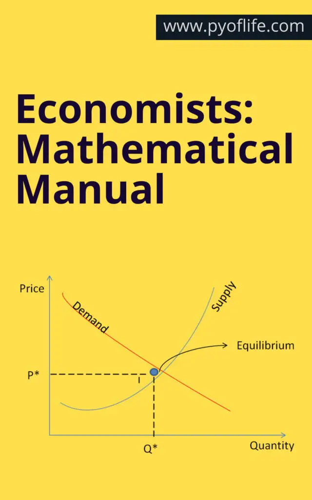
Economists: Mathematical Manual: Economics, often dubbed the “dismal science,” is far more vibrant and dynamic than this moniker suggests. At its core, economics is the study of how societies allocate scarce resources among competing uses. To understand and predict these allocations, economists rely heavily on mathematical tools and techniques. This article provides a comprehensive guide to the essential mathematical concepts and methods used in economics, aiming to serve as a handy reference for students, professionals, and enthusiasts alike.
Mathematics provides a formal framework for analyzing economic theories and models. It helps in deriving precise conclusions from assumptions and in rigorously testing hypotheses. The quantitative nature of economics makes mathematics indispensable for:
Formulating economic theories.
Analyzing data and interpreting results.
Making predictions about economic behavior.
Conducting policy analysis and evaluation.
Key Mathematical Concepts in Economics
1. Algebra and Linear Equations
Algebra forms the backbone of most economic analyses. Linear equations are particularly crucial as they represent relationships between variables in a simplified manner.
Example: The supply and demand functions in a market can be expressed as linear equations:
Qd=a−bPQ_d = a – bPQd=a−bP (Demand function)
Qs=c+dPQ_s = c + dPQs=c+dP (Supply function)
Where QdQ_dQd is the quantity demanded, QsQ_sQs is the quantity supplied, PPP is the price, and aaa, bbb, ccc, and ddd are parameters.
Calculus, particularly differentiation and integration, is fundamental in economics for understanding changes and trends.
Differentiation helps in finding the rate of change of economic variables. For example, marginal cost and marginal revenue are derivatives of cost and revenue functions, respectively.
Integration is used for aggregating economic quantities, such as finding total cost from marginal cost.
Example: If the total cost function is C(Q)=100+10Q+0.5Q2C(Q) = 100 + 10Q + 0.5Q^2C(Q)=100+10Q+0.5Q2, the marginal cost (MC) is the derivative MC=dCdQ=10+QMC = \frac{dC}{dQ} = 10 + QMC=dQdC=10+Q.
3. Optimization
Optimization techniques are crucial for decision-making in economics. Economists often seek to maximize or minimize objective functions subject to certain constraints.
Unconstrained Optimization: Solving problems without restrictions, typically by setting the derivative equal to zero to find critical points.
Constrained Optimization: Involves using methods like Lagrange multipliers to handle constraints.
Example: A firm wants to maximize its profit π=TR−TC\pi = TR – TCπ=TR−TC, where TRTRTR is total revenue and TCTCTC is the total cost. By differentiating π\piπ concerning quantity and setting it to zero, we find the optimal output level.
4. Matrix Algebra
Matrix algebra is used extensively in econometrics, input-output analysis, and in solving systems of linear equations.
Econometrics: Matrices simplify the representation and solution of multiple regression models.
Input-Output Analysis: Leontief models use matrices to describe the flow of goods and services in an economy.
Example: A simple econometric model can be written in matrix form as Y=Xβ+ϵY = X\beta + \epsilonY=Xβ+ϵ, where YYY is the vector of observations, XXX is the matrix of explanatory variables, β\betaβ is the vector of coefficients, and ϵ\epsilonϵ is the error term.
Econometric Techniques
Econometrics combines economic theory, mathematics, and statistical inference to quantify economic phenomena. Some essential techniques include:
1. Regression Analysis
Regression analysis estimates the relationships between variables. The most common is the Ordinary Least Squares (OLS) method.
Example: Estimating the consumption function C=α+βY+uC = \alpha + \beta Y + uC=α+βY+u, where CCC is consumption, YYY is income, and uuu is the error term.
2. Time Series Analysis
Time series analysis deals with data collected over time, essential for analyzing economic trends and forecasting.
Autoregressive (AR) Models: Explain a variable using its past values.
Moving Average (MA) Models: Use past forecast errors.
ARIMA Models: Combine AR and MA models to handle non-stationary data.
Example: GDP forecasting using an ARIMA model involves identifying the order of the model and estimating parameters to predict future values.
3. Panel Data Analysis
Panel data combines cross-sectional and time-series data, allowing for more complex analyses and control of individual heterogeneity.
Example: Studying the impact of education on earnings using data from multiple individuals over several years.
Game Theory
Game theory analyzes strategic interactions where the outcome depends on the actions of multiple agents. Key concepts include:
Nash Equilibrium: A situation where no player can benefit by changing their strategy unilaterally.
Dominant Strategies: A strategy that yields a better outcome regardless of what others do.
Example: The Prisoner’s Dilemma illustrates how rational individuals might not cooperate, even if it appears that cooperation would be beneficial.
Dynamic Programming
Dynamic programming solves complex problems by breaking them down into simpler sub-problems. It is particularly useful in macroeconomics and finance for:
Optimal Control Theory: Managing economic systems over time.
Bellman Equation: A recursive equation used in dynamic programming.
Example: Determining optimal investment strategies over time by maximizing the expected utility of consumption.
Economists: Mathematical Manual
Conclusion: Mathematics is the language through which economists describe, analyze, and interpret economic phenomena. From basic algebra to advanced econometric techniques, mathematical tools are indispensable for anyone seeking to understand or contribute to economics. This manual provides a glimpse into the essential mathematical methods used in economics. Still, continuous learning and practice are necessary to master these tools and apply them effectively in real-world scenarios.
Data science is a rapidly evolving field that leverages various techniques and tools to extract insights from data. R, a powerful and versatile programming language, is extensively used in data science for its statistical capabilities and comprehensive package ecosystem. This guide provides a detailed exploration of practical data science with R, from basic syntax to advanced machine learning and deployment.
What is Data Science?
Definition and Scope
Data science involves the use of algorithms, data analysis, and machine learning to interpret complex data and derive meaningful insights. It intersects various disciplines, including statistics, computer science, and domain-specific knowledge, to solve real-world problems.
Importance in Various Fields
Data science plays a crucial role across different sectors such as healthcare, finance, marketing, and government. It aids in making informed decisions, improving operational efficiency, and providing personalized experiences.
Overview of R Programming Language
History and Evolution
R was developed in the early 1990s by Ross Ihaka and Robert Gentleman at the University of Auckland, New Zealand. It evolved from the S language, becoming a favorite among statisticians and data miners for its extensive statistical libraries.
Why Choose R for Data Science?
R is favored for data science due to its vast array of packages, strong community support, and its powerful data handling and visualization capabilities. It excels in statistical analysis, making it a go-to tool for data scientists.
To begin with R, download and install R from CRAN (Comprehensive R Archive Network). For an enhanced development experience, install RStudio, an integrated development environment (IDE) that simplifies coding in R.
Configuring R for Data Science Projects
Proper configuration involves setting up necessary packages and libraries, customizing the IDE settings, and organizing your workspace for efficient project management.
Basic R Syntax and Data Types
Variables and Data Types
In R, data types include vectors, lists, matrices, data frames, and factors. Variables are created using the assignment operator <-. Understanding these basics is crucial for effective data manipulation and analysis.
Basic Operations in R
Basic operations involve arithmetic calculations, logical operations, and data manipulation techniques. Mastering these operations lays the foundation for more complex analyses.
Data Manipulation with dplyr
Introduction to dplyr
dplyr is a powerful package for data manipulation in R. It simplifies data cleaning and transformation with its intuitive syntax and robust functions.
Data Cleaning and Transformation
Using dplyr, data cleaning and transformation become streamlined tasks. Functions like filter(), select(), mutate(), and arrange() are essential for preparing data for analysis.
Aggregation and Summarization
dplyr also excels in aggregating and summarizing data. Functions such as summarize() and group_by() allow for efficient data summarization and insights extraction.
ggplot2, an R package, is renowned for its elegant and versatile data visualization capabilities. It follows the grammar of graphics, making it highly flexible and customizable.
Creating Various Types of Plots
With ggplot2, you can create a variety of plots, including scatter plots, line graphs, bar charts, and histograms. Each plot type serves different analytical purposes and helps in visual data exploration.
Customizing Plots
Customization in ggplot2 is extensive. You can modify plot aesthetics, themes, and scales to enhance the visual appeal and clarity of your data visualizations.
Descriptive statistics involve summarizing and describing the features of a dataset. R provides functions to calculate mean, median, mode, standard deviation, and other summary statistics.
Inferential Statistics
Inferential statistics allow you to make predictions or inferences about a population based on sample data. Techniques include confidence intervals, regression analysis, and ANOVA.
Hypothesis Testing
Hypothesis testing in R involves testing assumptions about data. Common tests include t-tests, chi-square tests, and ANOVA, which help in validating scientific hypotheses.
Machine learning (ML) in R involves using algorithms to build predictive models. R’s ML capabilities are enhanced by packages such as caret, randomForest, and xgboost.
Supervised Learning Algorithms
Supervised learning involves training a model on labeled data. Common algorithms include linear regression, logistic regression, decision trees, and support vector machines.
Unsupervised Learning Algorithms
Unsupervised learning deals with unlabeled data to find hidden patterns. Algorithms such as k-means clustering and principal component analysis (PCA) are widely used.
Text Mining and Natural Language Processing
Introduction to Text Mining
Text mining involves extracting meaningful information from text data. R provides several packages like tm and text mining tools for this purpose.
Techniques for Text Analysis
Text analysis techniques include tokenization, stemming, and lemmatization. These methods help in transforming raw text into analyzable data.
Sentiment Analysis
Sentiment analysis involves determining the sentiment expressed in a text. R packages like syuzhet and sentimentr facilitate this analysis, providing insights into public opinion.
Time series data is data that is collected at successive points in time. Understanding its characteristics is crucial for effective analysis and forecasting.
Forecasting Methods
Forecasting methods in R include ARIMA, exponential smoothing, and neural networks. These methods predict future values based on historical data.
Evaluating Forecast Accuracy
Evaluating the accuracy of forecasts involves using metrics like Mean Absolute Error (MAE) and Root Mean Squared Error (RMSE). These metrics assess the model’s predictive performance.
Working with Big Data in R
Introduction to Big Data Concepts
Big data involves large and complex datasets that traditional data processing techniques cannot handle. R’s integration with big data technologies makes it a valuable tool for big data analysis.
R Packages for Big Data
R packages such as dplyr, data.table, and sparklyr enable efficient handling and analysis of big data. These packages provide tools for data manipulation, visualization, and modeling.
Case Studies and Applications
Case studies in big data illustrate the practical applications of R in handling large datasets. Examples include analyzing social media data and sensor data from IoT devices.
Deploying Data Science Models
Introduction to Model Deployment
Model deployment involves putting machine learning models into production. This step is crucial for delivering actionable insights in real-time applications.
Tools and Techniques
R provides several tools for model deployment, including Shiny for web applications and plumber for creating APIs. These tools facilitate the integration of models into operational systems.
Case Studies
Case studies in model deployment showcase real-world applications. Examples include deploying predictive models in finance for credit scoring and in healthcare for patient diagnosis.
Collaborating and Sharing Work
Version Control with Git
Version control with Git is essential for collaborative data science projects. It allows multiple users to work on the same project simultaneously and maintain a history of changes.
Sharing Work through R Markdown
R Markdown enables the creation of dynamic documents that combine code, output, and narrative. It is an excellent tool for sharing reproducible research and reports.
Collaborating with Teams
Collaboration tools such as GitHub, Slack, and project management software enhance teamwork. Effective communication and project planning are key to successful data science projects.
Best Practices in Data Science Projects
Project Planning and Management
Effective project planning and management ensure that data science projects are completed on time and within budget. This involves defining clear goals, timelines, and deliverables.
Ethical Considerations
Ethical considerations in data science include data privacy, bias, and fairness. Adhering to ethical guidelines is crucial for maintaining trust and credibility.
Continuous Learning and Improvement
Continuous learning and improvement involve staying updated with the latest developments in data science. This includes attending conferences, taking courses, and participating in professional communities.
In healthcare, data science applications include predictive analytics for patient outcomes, personalized medicine, and operational efficiency improvements.
Case Study 2: Finance
In finance, data science is used for credit scoring, fraud detection, and algorithmic trading. These applications help in managing risks and optimizing investment strategies.
Case Study 3: Marketing
In marketing, data science aids in customer segmentation, sentiment analysis, and campaign optimization. It helps in understanding customer behavior and enhancing marketing effectiveness.
Advanced statistical methods include multivariate analysis, Bayesian statistics, and survival analysis. These methods address complex data scenarios and provide deeper insights.
Advanced Machine Learning Techniques
Advanced machine learning techniques involve deep learning, reinforcement learning, and ensemble methods. These techniques improve model accuracy and performance.
Specialized Packages and Tools
Specialized packages and tools in R cater to specific data science needs. Examples include Bioconductor for bioinformatics and rpart for recursive partitioning.
Resources for Learning R and Data Science
Books and Online Courses
Books and online courses provide structured learning paths for mastering R and data science. Popular resources include “R for Data Science” by Hadley Wickham and Coursera courses.
Communities and Forums
Communities and forums such as RStudio Community, Stack Overflow, and Kaggle offer support and knowledge sharing. Participating in these communities helps in solving problems and staying updated.
Continuous Learning Paths
Continuous learning paths involve a mix of formal education, online courses, and self-study. Keeping abreast of the latest research and trends is essential for career growth in data science.
Conclusion: Practical Data Science with R
Practical data science with R encompasses a wide range of techniques and tools for data manipulation, visualization, statistical analysis, machine learning, and deployment. Mastery of R provides a strong foundation for solving complex data problems and deriving actionable insights.
In today’s data-driven world, machine learning has become an indispensable tool across various industries. Machine learning algorithms allow systems to learn and make decisions from data without being explicitly programmed. This article explores pro machine learning algorithms, shedding light on their types, applications, and best practices for implementation.
What Are Machine Learning Algorithms?
Machine learning algorithms are computational methods that enable machines to identify patterns, learn from data, and make decisions or predictions. They are the backbone of artificial intelligence, powering applications ranging from simple email filtering to complex autonomous driving systems.
Types of Machine Learning Algorithms
Machine learning algorithms can be categorized into four main types: supervised learning, unsupervised learning, semi-supervised learning, and reinforcement learning. Each type has its own unique methodologies and applications.
Supervised learning algorithms are trained on labeled data, where the input and output are known. They are used for classification and regression tasks.
Linear Regression
Logistic Regression
Decision Trees
Support Vector Machines (SVM)
Neural Networks
Unsupervised Learning
Unsupervised learning algorithms deal with unlabeled data, finding hidden patterns and structures within the data.
K-Means Clustering
Hierarchical Clustering
Principal Component Analysis (PCA)
Independent Component Analysis (ICA)
Semi-Supervised Learning
Semi-supervised learning combines labeled and unlabeled data to improve learning accuracy.
Reinforcement learning algorithms learn by interacting with the environment, receiving rewards or penalties based on actions taken.
Q-Learning
Deep Q-Network (DQN)
Policy Gradient Methods
Actor-Critic Methods
Supervised Learning Algorithms
Supervised learning involves using known input-output pairs to train models that can predict outputs for new inputs. Here are some key supervised learning algorithms:
Linear Regression
Linear regression is used for predicting continuous values. It assumes a linear relationship between the input variables (features) and the single output variable (label).
Logistic Regression
Logistic regression is a classification algorithm used to predict the probability of a binary outcome. It uses a logistic function to model the relationship between the features and the probability of a particular class.
Decision Trees
Decision trees split the data into subsets based on feature values, creating a tree-like model of decisions. They are simple to understand and interpret, making them popular for classification and regression tasks.
Support Vector Machines (SVM)
SVMs are used for classification by finding the hyperplane that best separates the classes in the feature space. They are effective in high-dimensional spaces and for cases where the number of dimensions exceeds the number of samples.
Neural Networks
Neural networks are a series of algorithms that mimic the operations of a human brain to recognize patterns. They consist of layers of neurons, where each layer processes input data and passes it to the next layer.
Unsupervised Learning Algorithms
Unsupervised learning algorithms are used to find hidden patterns in data without pre-existing labels.
K-Means Clustering
K-Means clustering partitions the data into K distinct clusters based on feature similarity. It is widely used for market segmentation, image compression, and more.
Hierarchical Clustering
Hierarchical clustering builds a hierarchy of clusters either through a bottom-up (agglomerative) or top-down (divisive) approach. It is useful for data with nested structures.
Principal Component Analysis (PCA)
PCA reduces the dimensionality of data by transforming it into a new set of variables (principal components) that are uncorrelated and capture the maximum variance in the data.
Independent Component Analysis (ICA)
ICA is used to separate a multivariate signal into additive, independent components. It is often used in signal processing and for identifying hidden factors in data.
Semi-Supervised Learning Algorithms
Semi-supervised learning is a hybrid approach that uses both labeled and unlabeled data to improve learning outcomes.
Self-Training
In self-training, a model is initially trained on a small labeled dataset, and then it labels the unlabeled data. The newly labeled data is added to the training set, and the process is repeated.
Co-Training
Co-training involves training two models on different views of the same data. Each model labels the unlabeled data, and the most confident predictions are added to the training set of the other model.
Multi-View Learning
Multi-view learning uses multiple sources or views of data to improve learning performance. Each view provides different information about the instances, enhancing the learning process.
Reinforcement Learning Algorithms
Reinforcement learning algorithms learn by interacting with their environment and receiving feedback in the form of rewards or penalties.
Q-Learning
Q-Learning is a model-free reinforcement learning algorithm that aims to learn the quality of actions, telling an agent what action to take under what circumstances.
Deep Q-Network (DQN)
DQN combines Q-Learning with deep neural networks, enabling it to handle large and complex state spaces. It has been successful in applications like playing video games.
Policy Gradient Methods
Policy gradient methods directly optimize the policy by gradient ascent, improving the probability of taking good actions. They are effective in continuous action spaces.
Actor-Critic Methods
Actor-Critic methods combine policy gradients and value-based methods, where the actor updates the policy and the critic evaluates the action taken by the actor, improving learning efficiency.
Deep learning algorithms are a subset of machine learning that involve neural networks with many layers, enabling them to learn complex patterns in large datasets.
Convolutional Neural Networks (CNN)
CNNs are designed for processing structured grid data like images. They use convolutional layers to automatically and adaptively learn spatial hierarchies of features.
Recurrent Neural Networks (RNN)
RNNs are used for sequential data as they have connections that form cycles, allowing information to persist. They are widely used in natural language processing.
Long Short-Term Memory (LSTM)
LSTMs are a type of RNN that can learn long-term dependencies, solving the problem of vanishing gradients in traditional RNNs. They are effective in tasks like language modeling and time series prediction.
Generative Adversarial Networks (GANs)
GANs consist of two neural networks, a generator, and a discriminator, that compete with each other. The generator creates data, and the discriminator evaluates its authenticity, leading to high-quality data generation.
Ensemble Learning Algorithms
Ensemble learning combines multiple models to improve prediction performance and robustness.
Bagging
Bagging (Bootstrap Aggregating) reduces variance by training multiple models on different subsets of the data and averaging their predictions. Random Forests are a popular bagging method.
Boosting
Boosting sequentially trains models, each correcting the errors of its predecessor. It focuses on hard-to-predict cases, improving accuracy. Examples include AdaBoost and Gradient Boosting.
Stacking
Stacking combines multiple models by training a meta-learner to make final predictions based on the predictions of base models, enhancing predictive performance.
Evaluating Machine Learning Models
Evaluating machine learning models is crucial to understand their performance and reliability.
Accuracy
Accuracy measures the proportion of correct predictions out of all predictions. It is suitable for balanced datasets but may be misleading for imbalanced ones.
Precision and Recall
Precision measures the proportion of true positive predictions among all positive predictions, while recall measures the proportion of true positive predictions among all actual positives. They are crucial for imbalanced datasets.
F1 Score
The F1 Score is the harmonic mean of precision and recall, providing a balanced measure for evaluating model performance, especially in imbalanced datasets.
ROC-AUC Curve
The ROC-AUC curve plots the true positive rate against the false positive rate, and the area under the curve (AUC) measures the model’s ability to distinguish between classes.
Choosing the Right Algorithm
Choosing the right machine learning algorithm depends on several factors:
Problem Type
Different algorithms are suited for classification, regression, clustering, or dimensionality reduction problems. The nature of the problem dictates the algorithm choice.
Data Size
Some algorithms perform better with large datasets, while others are suitable for smaller datasets. Consider the data size when selecting an algorithm.
Interpretability
Interpretability is crucial in applications where understanding the decision-making process is important. Simple algorithms like decision trees are more interpretable than complex ones like deep neural networks.
Training Time
The computational resources and time available for training can influence the choice of algorithm. Some algorithms require significant computational power and time to train.
Practical Applications of Machine Learning Algorithms
Machine learning algorithms are applied in various fields, solving complex problems and automating tasks.
Healthcare
In healthcare, machine learning algorithms are used for disease prediction, medical imaging, and personalized treatment plans, improving patient outcomes and operational efficiency.
Finance
In finance, algorithms are used for fraud detection, algorithmic trading, and risk management, enhancing security and profitability.
Marketing
Machine learning enhances marketing efforts through customer segmentation, personalized recommendations, and predictive analytics, driving sales and customer engagement.
Autonomous Vehicles
Autonomous vehicles rely on machine learning algorithms for navigation, object detection, and decision-making, enabling safe and efficient self-driving technology.
Challenges in Machine Learning
Despite its potential, machine learning faces several challenges.
Data Quality
The quality of data impacts the performance of machine learning models. Noisy, incomplete, or biased data can lead to inaccurate predictions.
Overfitting and Underfitting
Overfitting occurs when a model learns the training data too well, capturing noise rather than the underlying pattern. Underfitting happens when a model fails to learn the training data adequately.
Computational Resources
Training complex models, especially deep learning algorithms, requires significant computational resources, which can be a barrier for some applications.
Future Trends in Machine Learning Algorithms
The field of machine learning is rapidly evolving, with several trends shaping its future.
Explainable AI
Explainable AI aims to make machine learning models transparent and interpretable, addressing concerns about decision-making in critical applications.
Quantum Machine Learning
Quantum machine learning explores the integration of quantum computing with machine learning, promising to solve complex problems more efficiently.
Automated Machine Learning (AutoML)
AutoML automates the process of applying machine learning to real-world problems, making it accessible to non-experts and accelerating model development.
Best Practices for Implementing Machine Learning Algorithms
Implementing machine learning algorithms requires adhering to best practices to ensure successful outcomes.
Data Preprocessing
Preprocessing involves cleaning and transforming data to make it suitable for modeling. It includes handling missing values, scaling features, and encoding categorical variables.
Feature Engineering
Feature engineering involves creating new features or transforming existing ones to improve model performance. It requires domain knowledge and creativity.
Model Validation
Model validation ensures that the model generalizes well to new data. Techniques like cross-validation and train-test splits help in evaluating model performance.
Case Studies of Successful Machine Learning Implementations
Several organizations have successfully implemented machine learning, demonstrating its potential.
AlphaGo by Google DeepMind
AlphaGo, developed by Google DeepMind, used reinforcement learning and neural networks to defeat world champions in the game of Go, showcasing the power of advanced algorithms.
Netflix Recommendation System
Netflix uses collaborative filtering and deep learning algorithms to provide personalized movie and TV show recommendations, enhancing user experience and retention.
Fraud Detection by PayPal
PayPal employs machine learning algorithms to detect fraudulent transactions in real-time, improving security and reducing financial losses.
Conclusion
Pro machine learning algorithms are transforming industries by enabling intelligent decision-making and automation. Understanding their types, applications, and best practices is crucial for leveraging their full potential. As technology evolves, staying updated with trends and advancements will ensure continued success in the ever-evolving field of machine learning.
Introductory Time Series with R: Time series analysis is a powerful statistical tool used to analyze time-ordered data points. This analysis is pivotal in various fields like finance, economics, environmental science, and more. With the advent of advanced computing tools, R programming has become a popular choice for time series analysis due to its extensive libraries and user-friendly syntax. This guide will delve into the basics of time series analysis using R, providing a solid foundation for beginners and a refresher for seasoned analysts.
Understanding Time Series
Definition of Time Series
A time series is a sequence of data points collected or recorded at specific time intervals. These data points represent the values of a variable over time, enabling analysts to identify trends, patterns, and anomalies.
Components of Time Series
Trend: The long-term movement or direction in the data.
Seasonality: Regular patterns or cycles in the data occurring at specific intervals.
Cyclicity: Fluctuations in data occurring at irregular intervals, often related to economic or business cycles.
Randomness: Irregular, unpredictable variations in the data.
To start with time series analysis in R, you need to install R and RStudio. R is the programming language, and RStudio is an integrated development environment (IDE) that makes R easier to use.
Installing Required Packages
For time series analysis, several R packages are essential. Some of these include:
forecast: For forecasting time series.
tseries: For time series analysis.
xts and zoo: For handling irregular time series data.
Evaluate the performance of your time series models using metrics like Mean Absolute Error (MAE), Mean Squared Error (MSE), and Root Mean Squared Error (RMSE).
accuracy(forecasted)
Cross-Validation
Cross-validation helps in assessing how the results of a statistical analysis will generalize to an independent data set.
Time series analysis is extensively used in financial market analysis for predicting stock prices, market trends, and economic indicators.
Weather Forecasting
Meteorologists use time series analysis to predict weather patterns and climate changes.
Demand Forecasting
Businesses use time series analysis for inventory management and predicting future demand.
Challenges in Time Series Analysis
Handling Missing Data
Missing data can distort the analysis. Techniques like interpolation, forward filling, and imputation can handle missing values.
Dealing with Outliers
Outliers can significantly affect the results. Identifying and handling outliers is crucial.
Choosing the Right Model
Selecting the appropriate model depends on the data’s nature and the analysis’s specific requirements.
Conclusion: Introductory Time Series with R
Time series analysis is critical for data analysts and scientists, offering valuable insights into temporal data. With R’s powerful libraries and tools, performing time series analysis becomes more accessible and efficient. By mastering the basics and exploring advanced techniques, you can unlock the full potential of time series data to inform decisions and predictions.
Python For Data Analysis: A Complete Guide For Beginners, Including Python Statistics And Big Data Analysis: Data analysis is a critical skill in today’s data-driven world. Whether you’re working in business, academia, or tech, understanding how to analyze data can significantly impact decision-making and strategy. Python, with its simplicity and powerful libraries, has become the go-to language for data analysis. This guide will walk you through everything you need to know to get started with Python for data analysis, including Python statistics and big data analysis.
Getting Started with Python
Before diving into data analysis, it’s crucial to set up Python on your system. Python can be installed from the official website. For data analysis, using an Integrated Development Environment (IDE) like Jupyter Notebook, PyCharm, or VS Code can be very helpful.
Installing Python
To install Python, visit the official Python website, download the installer for your operating system, and follow the installation instructions.
IDEs for Python
Choosing the right IDE can enhance your productivity. Jupyter Notebook is particularly popular for data analysis because it allows you to write and run code in an interactive environment. PyCharm and VS Code are also excellent choices, offering advanced features for coding, debugging, and project management.
Basic Syntax
Python’s syntax is designed to be readable and straightforward. Here’s a simple example:
# This is a comment
print("Hello, World!")
Understanding the basics of Python syntax, including variables, data types, and control structures, will be foundational as you delve into data analysis.
Python’s ecosystem includes a vast array of libraries tailored for data analysis. These libraries provide powerful tools for everything from numerical computations to data visualization.
Introduction to Libraries
Libraries like Numpy, Pandas, Matplotlib, Seaborn, and Scikit-learn are essential for data analysis. Each library has its specific use cases and advantages.
Installing Libraries
Installing these libraries is straightforward using pip, Python’s package installer. For example:
Numpy: Ideal for numerical operations and handling large arrays.
Pandas: Perfect for data manipulation and analysis.
Matplotlib and Seaborn: Great for creating static, animated, and interactive visualizations.
Scikit-learn: Essential for implementing machine learning algorithms.
Numpy for Numerical Data
Numpy is a fundamental library for numerical computations. It provides support for arrays, matrices, and many mathematical functions.
Introduction to Numpy
Numpy allows for efficient storage and manipulation of large datasets.
Creating Arrays
Creating arrays with Numpy is simple:
import numpy as np

# Creating an array
array = np.array([1, 2, 3, 4, 5])
print(array)
Array Operations
Numpy supports various operations like addition, subtraction, multiplication, and division on arrays. These operations are element-wise, making them efficient for large datasets.
EDA involves analyzing datasets to summarize their main characteristics, often using visual methods.
Importance of EDA
EDA helps in understanding the structure of data, detecting outliers, and uncovering patterns.
Descriptive Statistics
Descriptive statistics summarize the central tendency, dispersion, and shape of a dataset’s distribution.
# Descriptive statistics
df.describe()
Visualizing Data
Visualizations can reveal insights that are not apparent from raw data.
# Visualizing data
sns.pairplot(df)
plt.show()
Statistical Analysis with Python
Statistics is a crucial part of data analysis, helping in making inferences and decisions based on data.
Introduction to Statistics
Statistics provides tools for summarizing data and making predictions.
Hypothesis Testing
Hypothesis testing is used to determine if there is enough evidence to support a specific hypothesis.
from scipy import stats

# Performing a t-test
t_stat, p_value = stats.ttest_1samp(df['Age'], 30)
print(p_value)
Regression Analysis
Regression analysis helps in understanding the relationship between variables.
import statsmodels.api as sm

# Performing linear regression
X = df['Age']
y = df['Name']
X = sm.add_constant(X)
model = sm.OLS(y, X).fit()
print(model.summary())
Machine Learning Basics
Machine learning involves training algorithms to make predictions based on data.
Introduction to Machine Learning
Machine learning is a subset of artificial intelligence focused on building models from data.
Common algorithms include linear regression, decision trees, and k-means clustering.
from sklearn.linear_model import LinearRegression

# Simple linear regression
model = LinearRegression()
model.fit(X, y)
print(model.coef_)
Handling Big Data with Python
Big data refers to datasets that are too large and complex for traditional data-processing software.
Introduction to Big Data
Big data requires specialized tools and techniques to store, process, and analyze.
Tools for Big Data
Hadoop and Spark are popular tools for handling big data.
Working with Large Datasets
Python libraries like Dask and PySpark can handle large datasets efficiently.
import dask.dataframe as dd

# Loading a large dataset
df = dd.read_csv('large_dataset.csv')
Case Study: Analyzing a Real-World Dataset
Applying the concepts learned to a real-world dataset can solidify your understanding.
Introduction to Case Study
Case studies provide practical experience in data analysis.
Dataset Overview
Choose a dataset that interests you and provides enough complexity for analysis.
Step-by-Step Analysis
Go through the steps of data cleaning, exploration, analysis, and visualization.
Python for Time Series Analysis
Time series analysis involves analyzing time-ordered data points.
Introduction to Time Series
Time series data is ubiquitous in fields like finance, economics, and weather forecasting.
Time Series Decomposition
Decomposition helps in understanding the underlying patterns in time series data.
from statsmodels.tsa.seasonal import seasonal_decompose

# Decomposing time series
result = seasonal_decompose(time_series, model='additive')
result.plot()
Forecasting Methods
Methods like ARIMA and exponential smoothing can be used for forecasting.
from statsmodels.tsa.arima.model import ARIMA

# ARIMA model
model = ARIMA(time_series, order=(5, 1, 0))
model_fit = model.fit()
print(model_fit.summary())
Python for Text Data Analysis
Text data analysis involves processing and analyzing text data to extract meaningful insights.
Introduction to Text Data
Text data is unstructured and requires specialized techniques for analysis.
Text Preprocessing
Preprocessing steps include tokenization, stemming, and removing stop words.
from nltk.tokenize import word_tokenize

# Tokenizing text
text = "This is an example sentence."
tokens = word_tokenize(text)
print(tokens)
Sentiment Analysis
Sentiment analysis helps in understanding the emotional tone of text.
from textblob import TextBlob

# Sentiment analysis
blob = TextBlob("I love Python!")
print(blob.sentiment)
Working with APIs and Web Scraping
APIs and web scraping allow you to gather data from the web for analysis.
Introduction to APIs
APIs provide a way to interact with web services and extract data.
Web Scraping Techniques
Web scraping involves extracting data from websites using libraries like BeautifulSoup and Scrapy.
import requests
from bs4 import BeautifulSoup

# Scraping a webpage
response = requests.get('https://example.com')
soup = BeautifulSoup(response.text, 'html.parser')
print(soup.title)
Handling Scraped Data
Clean and structure the scraped data for analysis.
Integrating SQL with Python
SQL is a standard language for managing and manipulating databases.
Introduction to SQL
SQL is used for querying and managing relational databases.
Connecting to Databases
Use libraries like SQLite and SQLAlchemy to connect Python to SQL databases.
import sqlite3

# Connecting to a database
conn = sqlite3.connect('database.db')
cursor = conn.cursor()
Performing SQL Queries
Execute SQL queries to retrieve and manipulate data.
# Executing a query
cursor.execute('SELECT * FROM table_name')
rows = cursor.fetchall()
print(rows)
Best Practices for Python Code in Data Analysis
Writing clean and efficient code is crucial for successful data analysis projects.
Writing Clean Code
Follow best practices like using meaningful variable names, commenting code, and following PEP 8 guidelines.
Version Control
Use version control systems like Git to manage your codebase.
Code Documentation
Documenting your code helps in maintaining and understanding it.
Python in Data Analysis Projects
Applying Python in real-world projects helps in gaining practical experience.
Project Workflow
Follow a structured workflow from data collection to analysis and visualization.
Planning and Execution
Plan your projects carefully and execute them systematically.
Real-World Project Examples
Look at examples of successful data analysis projects for inspiration.
Common Challenges and Solutions
Data analysis projects often come with challenges. Knowing how to overcome them is crucial.
Common Issues
Issues can range from missing data to performance bottlenecks.
Troubleshooting
Develop a systematic approach to debugging and solving problems.
Optimization Techniques
Optimize your code for better performance, especially when dealing with large datasets.
Future of Python in Data Analysis
Python continues to evolve, and its role in data analysis is becoming more significant.
Emerging Trends
Keep an eye on emerging trends like AI and machine learning advancements.
Python’s Evolving Role
Python’s libraries and tools are constantly improving, making it even more powerful for data analysis.
Career Opportunities
Data analysis skills are in high demand across various industries. Mastering Python can open up numerous career opportunities.
Conclusion: Python For Data Analysis: A Complete Guide For Beginners, Including Python Statistics And Big Data Analysis
Python is a versatile and powerful tool for data analysis. From basic data manipulation to advanced statistical analysis and machine learning, Python’s extensive libraries and user-friendly syntax make it accessible for beginners and powerful for experts. By mastering Python for data analysis, you can unlock valuable insights from data and drive impactful decisions in any field.