Data Science Archives - Page 43 of 45

Simple R Studio Hack That You Should Know

Simple R Studio Hack That You Should Know: RStudio is an open-source tool for programming in R. If you are interested in programming with R, it’s worth knowing about the capabilities of RStudio. It is a flexible tool that helps you create readable analyses and keeps your code, images, comments, and plots together in one place. In this article, we are going to talk about an R studio hack that every R user should know:

1. Keyboard Shortcuts

If you know RStudio keyboard shortcuts will save lots of time when programming. RStudio provides dozens of useful shortcuts that you can access through the menu at the top: Tools > Keyboard Shortcuts Help. Another way to access RStudio keyboard shortcuts is with a shortcut! To access shortcuts, type Option + Shift + K on a Mac or

Here are some of our favorite RStudio shortcuts:

Insert the <- assignment operator with Option + - on a Mac, or Alt + - on Linux and Windows.
Insert the pipe operator %>% with Command + Shift + M on a Mac, or Ctrl + Shift + M on Linux and Windows.
Run the current line of code with Command + Enter on a Mac or Control + Enter on Linux and Windows.
Run all lines of code with Command + A + Enter on a Mac or Control + A + Enter on Linux and Windows.
Restart the current R session and start fresh with Command + Shift + F10 on a Mac or Control + Shift + F10 on Linux and Windows.

Another excellent resource for RStudio shortcuts is the official RStudio cheat sheet.

2. Customize the Appearance

RStudio offers a wealth of options to customize the appearance to your liking. Under the RStudio tab, navigate to Preferences > Appearance to explore the many options available. A nice feature of RStudio is that you can quickly click through the Editor theme window to preview each theme.

3. Manage Version Control with GitHub in RStudio

In addition to managing packages in RStudio, you can also use GitHub with RStudio to maintain version control of your projects and R scripts. Check out this article from GitHub and this article from RStudio for all the information you need to integrate Git into your RStudio workflow.

4. Preview and Save Your Plots

Plots generated during an RStudio session are displayed under the Plots tab in the lower-right window. In this window, you can inspect your plots by zooming in and out. If you want to save your plot, you can save the plot as a PDF or image file.

5. Organize Your Work with Projects

RStudio offers a powerful feature to keep you organized; Projects. It is important to stay organized when you work on multiple analyses. Projects from RStudio allow you to keep all of your important work in one place, including code scripts, plots, figures, results, and datasets. Create a new project by navigating to the File tab in RStudio and selecting New Project… You have the option to create your new project in a new directory or an existing directory.

RStudio offers dedicated project types if you are working on an R package or a Shiny Web Application. RStudio Projects are useful when you need to share your work with colleagues. You can send your project file (ending in .Rproj) along with all supporting files, which will make it easier for your colleagues to recreate the working environment and reproduce the results.

6. Manage Package Versions with renv

We love R at Dataquest, but managing package versions can be a challenge! Fortunately, R package management is easier than ever, thanks to the renv (“reproducible environment”) package from RStudio. And now, RStudio includes built-in support for renv. We won’t get into the details of how to use renv with RStudio projects in this blog because RStudio provides you with the info you need in the link we provided and in the vignette. But using renv with RStudio can make R package management much easier, so we wanted to let you know!

The renv the package is replacing the Packrat package that RStudio used to maintain. To use the renv package with your RStudio projects upgrade to the latest version of RStudio and then install the renv package with library("renv"). From there you will have the option to use renv it with all new projects.

7. Easy Links to Documentation

Under the Help tab in the lower-right window, you’ll find handy links to the online documentation for R functions and R packages. For example, if we search for information about the install.packages() function using the search bar, the official documentation is returned:

We can also access documentation in the Help tab by prepending a package or function with ?, (e.g. ?install.packages) and running the command into the Console. With either approach, RStudio auto-fills matching function names as you type.

October 18, 2022 by SAROJ Data Science

R Cheat Sheet For Everyone

R is a powerful programming language used for data analysis and statistical computing. Here is a quick reference guide to get you started with R programming.

Basic Syntax:

Comments start with the “#” symbol
Assignment operator is “<-“
Function calls use parentheses, e.g. mean(x)
“print()” function can be used to display results
Use “?” before a function to get help, e.g. ?mean

Data Types:

Numeric: numbers with decimal places, e.g. 3.14
Integer: whole numbers, e.g. 5
Character: text, e.g. “hello”
Factor: categorical data, e.g. “male” or “female”
Logical: binary values, either TRUE or FALSE

Vectors:

A vector is a collection of values with the same data type
Creation of vectors using c(), e.g. c(1,2,3)
Use “[]” to access elements of a vector, e.g. x[2]
Use “length()” to get the number of elements in a vector

Matrices:

A matrix is a 2-dimensional vector with rows and columns
Creation of matrices using matrix(), e.g. matrix(1:9, ncol=3)
Use “[row, col]” to access elements of a matrix, e.g. m[2,3]
Use “dim()” to get the dimensions of a matrix

DataFrames:

A data frame is a 2-dimensional data structure with rows and columns
Creation of data frames using data.frame(), e.g. data.frame(x=1:5, y=6:10)
Use “$” to access columns of a data frame, e.g. df$x
Use “nrow()” and “ncol()” to get the number of rows and columns

Reading Data:

Use read.csv() to read csv files, e.g. read.csv(“data.csv”)
Use read.table() to read other types of files, e.g. read.table(“data.txt”, sep=”\t”)

Data Manipulation:

Use “head()” and “tail()” to view the first and last few rows of a data frame
Use “subset()” to extract a subset of a data frame based on conditions, e.g. subset(df, x > 3)
Use “merge()” to combine two data frames based on common columns

Plotting:

Use “plot()” to create basic plots, e.g. plot(x, y)
Use “hist()” to create histograms, e.g. hist(x)
Use “boxplot()” to create box plots, e.g. boxplot(x)
Use “barplot()” to create bar plots, e.g. barplot(x)

Statistics:

Use “mean()” to calculate the mean of a vector, e.g. mean(x)
Use “median()” to calculate the median of a vector, e.g. median(x)
Use “sd()” to calculate the standard deviation of a vector, e.g. sd(x)
Use “summary()” to get a summary of a data frame, e.g. summary(df)

Download A Complete PDF

October 12, 2022 by SAROJ Data Science

Download Python Cheat Sheet

Python cheat sheet can be an essential tool for anyone looking to learn or improve their skills in this powerful and versatile programming language. Whether you’re just starting out or you’re an experienced developer, a Python cheat sheet is a handy reference that can help you quickly and easily find the information you need to write your code. In this article, we’ll explore some of the key features of Python and provide you with a comprehensive Python cheat sheet that you can use to get up and running quickly.

Download (PDF)

Basic Syntax: Python uses indentation to define blocks of code, and its syntax is straightforward and easy to read. The print statement is used to output data to the console, and variables can be defined using the assignment operator (=).

Data Types: Python supports several data types, including integers, floating-point numbers, strings, and lists. There are also several built-in functions and methods that allow you to manipulate and analyze data, such as len(), min(), max(), and sorted().

Operators: Python supports several basic arithmetic operators, such as +, -, *, and /, as well as comparison operators like <, >, and ==. There are also several logical operators, such as and, or, and not, which can be used to control the flow of your code.

Control Flow: Python uses if-elif-else statements to control the flow of your code, and there are also several built-in functions, such as range(), that can be used to loop through data. Additionally, there are several built-in functions for working with arrays and lists, such as sorted(), reversed(), and enumerate().

Functions: Functions are an important part of any programming language, and Python is no exception. Functions can be defined using the def keyword, and they can accept parameters and return values. There are also several built-in functions, such as len(), that can be used to manipulate data.

Libraries: Python is widely used for data analysis, and there are several libraries, such as NumPy and Pandas, that provide tools for working with data. Additionally, there are several libraries for machine learning and artificial intelligence, such as TensorFlow and scikit-learn, that can be used to build sophisticated models.

Here is a comprehensive Python cheat sheet that summarizes the key features of Python:

Basic syntax:

Use indentation to define blocks of code
The print statement is used to output data to the console
Variables are defined using the assignment operator (=)

Data types:

Integers
Floating-point numbers
Strings
Lists
Built-in functions and methods for manipulating and analyzing data

Operators:

Arithmetic operators: +, -, *, /
Comparison operators: <, >, ==
Logical operators: and, or, not

Control flow:

if-elif-else statements
Built-in functions for looping through data: range()
Built-in functions for working with arrays and lists: sorted(), reversed(), enumerate()

Functions:

Defined using the def keyword
Can accept parameters and return values
Built-in functions for manipulating data: len()

Libraries:

NumPy and Pandas for data analysis
TensorFlow and scikit-learn for machine learning and artificial intelligence.

October 12, 2022 by SAROJ Books Data Science

Top R Packages For Data Visualization That You Should know

Top R Packages For Data Visualization That You Should Know: The popular data visualization tools that are available are Tableau, Plotly, R, Google Charts, Infogram, and Kibana. The various data visualization platforms have different capabilities, functionality, and use cases. They also require a different skill set. This article discusses the use of the top R packages for data visualization. R is a language that is designed for statistical computing, graphical data analysis, and scientific research. As per study reports, data scientists and practitioners prefer R as the language for statistical modeling. Also, R dominates the preference scale, with a combined figure of 81.9% utilization for statistical modeling among those surveyed.

Below here, we listed the top R packages for data visualization that you should know:

1. GGPLOT2

While it’s relatively easy to create standard plots in R, if you need to make a custom plot, things can get hairy fast. That’s why ggplot2 was born: to make building custom plots easier. ggplot2 is based on The Grammar of Graphics, a system for understanding graphics as composed of various layers that together create a complete plot. With ggplot2, you can, for instance, start building your plot with axes, then add points, then a line, a confidence interval, and so on. The drawback of ggplot2 is that it may be slower than base R, and new programmers may find the learning curve to be a bit steep.

2. Colourpicker

Colourpicker is a tool for the Shiny framework and for selecting colours in plots. This tool supports various options, such as alpha opacity, custom colour palettes, and more. The most common uses of this tool include the utilisation of the colourInput() function to create a colour input in Shiny as well as the use of the plotHelper() function/RStudio Addin to select colours for a plot.

3. Highcharter

Highcharter makes dynamic charting easy. It uses a single function, hchart(), to draw plots for all kinds of R object classes, from data frame to dendrogram to phylo. It also gives R coders a handy way to access the other popular Highcharts plot types, Highstock (for financial charting) and Highmaps (for schematic maps in web-based projects). The package has easy-to-customize themes, along with built-in themes like “economist,” “financial times,” and “538,” in case you want to borrow a look for your chart from the pros.

4. Esquisse

The esquisse package allows a user to interactively explore data by visualising it with the ggplot2 package. It allows a user to draw bar graphs, curves, scatter plots, and histograms, export the graphs, and retrieve the code generating the graph. With the help of esquisse, one can quickly visualise the data according to their type, export it to PNG or PowerPoint, and retrieve the code to reproduce the chart.

5. Plotly

You might know Plotly as an online platform for data visualization, but did you know you can access its capabilities from an R or Python Notebook? Like highcharter, Plotly’s forte is making interactive plots, but it offers some charts you won’t find in most packages, like contour plots, candlestick charts, and 3D charts.

6. Quantmod

Quantmod is an R package that provides a framework for quantitative financial modelling and trading. It provides a rapid prototyping environment that makes modelling easier by removing the repetitive workflow issues surrounding data management and visualisation.

7. Leaflet

Leaflet offers a lightweight but powerful way to build interactive maps, which you’ve probably seen in action (in their JS form) on sites ranging from The New York Times and The Washington Post to GitHub and GIS specialists like Mapbox and CartoDB. The R interface for Leaflet was developed using the htmlwidgets framework, which makes it easy to control and integrate Leaflet maps right in R Markdown documents (v2), RStudio, or Shiny apps.

September 21, 2022 by SAROJ Books Data Science

Advantages of Using R for Data Science

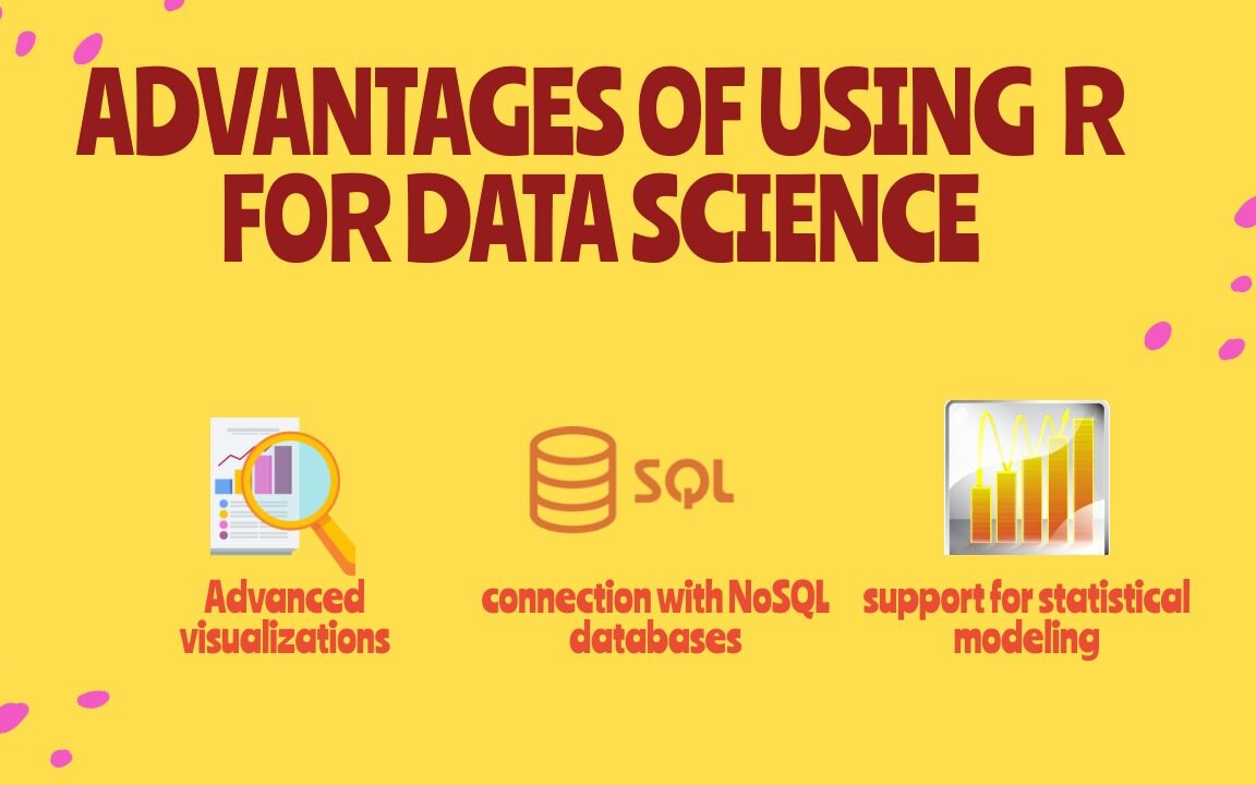
Advantages of Using R for Data Science, In modern times, the field of data science is evolving at a breakneck pace. Hence, businesses need to embrace the same before getting left behind at a distance that will keep on increasing over time. R is a powerful tool that has excellent statistical and visualization capabilities, making it very attractive to data scientists.

R is the most powerful tool to execute algorithms related to data science and has the capability of working with abundant data. It provides a wide variety of linear and non-linear models, classical statistical tests, time series analysis and machine learning capabilities (i.e., classification, clustering, regression, and reinforcement learning), and excellent visualization techniques.

5 Advantages of Using R for Data Science

1) Free and Open Source

An open-source language is a language on which we can work without needing a license or a fee. R is an open-source language. We can contribute to the development of R by optimizing our packages, developing new ones, and resolving issues.

2) Extensive support for statistical modeling

Statistical modeling is essential to determine how one variable is related to others. R provides powerful capabilities to deal with statistical modeling. It has excellent functions for central tendency, the measure of variability, probability, hypothesis testing, ANOVA, and regression analysis.

3) Extremely easy data wrangling

R has several packages that hugely simplify the process of preparing your data for analysis. You may have your data stored in the .csv or .txt file, in Excel spreadsheets, in relational databases, or as a SAS or Stata file. R can load these various types of files with just one line of code.

The process of data cleaning and transforming is also straightforward. One line of code – and you create a separate dataset without any missing values, another line – and you impose multiple filters on your data. With such powerful capabilities, the time you spend preparing your data for analysis can decrease significantly, giving you more time to spend it on the analysis itself.

4) The connection with NoSQL databases

The majority of data science projects deal with unstructured data. R can provide interfaces with NoSQL databases and analyze unstructured data in effective ways.

5) Advanced visualizations

Even the basic functionality of R allows you to create histograms, scatterplots, or line plots with only a tiny bit of code. These are very convenient functions for visualizing your data before even starting any analysis. In a few seconds, you can see your data and get insights that are not visible from the tabulated data alone.

However, if you spend some time learning more advanced visualization packages, such as ggplot2, for example, you’ll be able to build some very impressive graphs. R provides seemingly countless ways to visualize your data. These graphs will look very professional. And you’ll get access to a whole host of extra options, such as adding maps to your visualizations or making them animated.

September 10, 2022 by SAROJ Data Science

How to Choose the Right Data Visualization

How to Choose the Right Data Visualization is divided into chapters, one for each of the main categories for using data visualization. Each chapter is headed by a short introduction and a list of chart types falling into that category. Each chart type is accompanied by a brief description and one or more icons. Below is a key for decoding these symbols:

BASIC: Chart types with this icon represent typical or standard chart types. When you need to create a data visualization, try to see if one of these chart, types works first, before deciding on an uncommon or advanced type.
UNCOMMON: Chart types with this icon are slightly more unusual than the most common chart types. Use cases for these charts are more specialized than other chart types in that same category or more frequently seen in other roles.
ADVANCED: Chart types with this icon are even more specialized in their roles. Make sure that the chart type is the best one for your use case before implementing it. Sometimes, these chart types will not be built into visualization software or libraries, and additional work will need to be done to put these types of charts together.

Download a pdf

How to Choose the Right Data Visualization

Follow us on Facebook: https://www.facebook.com/pyoflife

August 24, 2022 by SAROJ Books Data Science

Solving a System of Equations in R With Examples

Solving a System of Equations in R With Examples: Solving a system of equations in R is a common task in mathematical and statistical applications. R has several built-in functions and packages to solve systems of equations, including the lm() function and the ‘rootSolve’ package. In this article, we will demonstrate how to solve a system of equations in R using these tools, with examples.

Example 1: Solving a System of Linear Equations with lm() Function

The lm() function can be used to solve a system of linear equations, where the equation can be represented in the form of y = mx + b, where m is the slope and b is the y-intercept. Let’s consider the following system of two linear equations:

y = 2x + 1

y = -x + 3

To solve this system of equations using lm() function, we first have to create a data frame to represent the equations, and then use the lm() function to fit a linear model to the data.

Creating a data frame to represent the equations

df <- data.frame(x = c(1, 2, 3), y = c(3, 5, 7))

Fitting a linear model to the data

lm_fit <- lm(y ~ x, data = df)

Extracting the coefficients of the model

coeffs <- coefficients(lm_fit)

Solving for x and y

x <- -(coeffs[1]/coeffs[2]) y <- coeffs[1] + coeffs[2] * x

Printing the solution

cat(“The solution is x =”, x, “and y =”, y)

The output will be:

The solution is x = 1.5 and y = 4

Example 2: Solving a Non-Linear System of Equations with rootSolve Package

The rootSolve package can be used to solve a non-linear system of equations, where the equations are not represented in the form of y = mx + b. Let’s consider the following system of two non-linear equations:

x^2 + y^2 = 1

x + y = 1

To solve this system of equations using rootSolve package, we first have to install and load the package, and then use the uniroot() function to find the solution.

Installing and loading the rootSolve package

install.packages(“rootSolve”) library(rootSolve)

Defining the system of equations

equations <- function(z) { x <- z[1] y <- z[2] f1 <- x^2 + y^2 – 1 f2 <- x + y – 1 c(f1, f2) }

Solving for x and y

solution <- uniroot(equations, c(-1, -1))

Printing the solution

cat(“The solution is x =”, solution$root[1], “and y =”, solution$root[2])

The output will be:

The solution is x = 0.5 and y = 0.5

Solving a system of equations in R is a straightforward task with the help of built-in functions and packages such as lm() and rootSolve. These functions can be used to solve both linear and non-linear systems of equations and provide accurate solutions for real-world problems.

August 1, 2022 by SAROJ Data Science

MOST COMMON STATISTICAL DISTRIBUTIONS

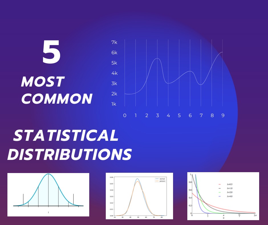
MOST COMMON STATISTICAL DISTRIBUTIONS: Statistics is an essential branch of mathematics that involves the collection, analysis, and interpretation of data. One of the central concepts in statistics is the idea of a distribution, which is a mathematical model that describes the pattern of the data. There are several common statistical distributions that are widely used in different areas of research and industry.

Normal Distribution: Also known as Gaussian Distribution, the normal distribution is a bell-shaped curve that represents the frequency of the data. It is commonly used to describe the distribution of continuous data that is symmetrical and follows a central tendency. The normal distribution is widely used in many fields, such as biology, finance, and psychology, to model the behavior of data.
Binomial Distribution: The binomial distribution is used to model the distribution of binary data, where there are only two possible outcomes. It is often used in medical trials, where the trial outcome can be either positive or negative. The binomial distribution is characterized by two parameters, n, and p, where n is the number of trials, and p is the probability of success in each trial.
Poisson Distribution: The Poisson distribution is used to model the number of events that occur in a fixed interval of time or space. It is often used in quality control, where the number of defects in a manufactured product is considered. The Poisson distribution is characterized by a single parameter, λ, which represents the average number of events in the interval.
Exponential Distribution: The exponential distribution is used to model the time between events in a Poisson process. It is often used in reliability engineering, where the time to failure of a device is modeled. The exponential distribution is characterized by a single parameter, λ, which represents the rate of events.
Log-Normal Distribution: The log-normal distribution is used to model data that is skewed to the right and has a heavy tail. It is often used in finance, where the distribution of stock prices is modeled. The log-normal distribution is characterized by two parameters, μ, and σ, which represent the mean and standard deviation of the logarithm of the data.

These are some of the most commonly used statistical distributions in various fields of research and industry. Understanding these distributions is essential for making informed decisions based on data. By knowing the pattern of the data, researchers can make predictions, test hypotheses, and draw conclusions about the population.

April 21, 2022 by SAROJ Data Science

R Programming Cheat Sheet For Basics Level

With the help of the R programming cheat sheet, we can perform a wide variety of statistical (linear and nonlinear modelling, classical statistical tests, time-series analysis, classification, clustering, …) and graphical techniques, and is highly extensible.

One of R’s strengths is the ease with which well-designed publication-quality plots can be produced, including mathematical symbols and formulae where needed. Great care has been taken over the defaults for the minor design choices in graphics, but the user retains full control.

Download R Cheatsheet

R Programming Cheat Sheet For Basics Level

January 20, 2022 by SAROJ Data Science

R Libraries Every Data Scientist Should Know

I have been using R for the longest time in my professional life, I realized that R outclasses Python in several use cases, particularly for statistical analyses. As well, R has some powerful packages that were built by the world’s biggest tech companies, and they aren’t in Python! And so, in this article, I wanted to go over three R packages that I highly recommend that you take the time to learn and add to your arsenal of tools because they are seriously powerful tools. Without further ado, here are three R packages that every data scientist should know:

1. Causal Impact (Google)

The package is designed to make a counterfactual inference as easy as fitting a regression model, but much more powerful, provided the assumptions above are met. The package has a single entry point, the function CausalImpact(). Given a response time series and a set of control time series, the function constructs a time-series model, performs posterior inference on the counterfactual, and returns an CausalImpact object. The results can be summarized in terms of a table, a verbal description, or a plot.

2. Robyn (Meta / Facebook)

Robyn is an automated Marketing Mix Modeling (MMM) code. It aims to reduce human bias by means of ridge regression and evolutionary algorithms, enables actionable decision making provides a budget allocator and diminishing returns curves and allows ground-truth calibration to account for causation

3. Anomaly Detection (Twitter)

AnomalyDetection is an open-source R package to detect anomalies that is robust, from a statistical standpoint, in the presence of seasonality and an underlying trend. The anomaly detection package can be used in a wide variety of contexts. For example, detecting anomalies in system metrics after a new software release, user engagement post an A/B test, or problems in econometrics, financial engineering, political and social sciences.

Download: Data Science with R: A Step-by-Step Guide

December 2, 2021 by SAROJ Data Science

Data Science

Below here, we listed the top R packages for data visualization that you should know:

5 Advantages of Using R for Data Science

Recent Posts

Books