An Introduction To R For Spatial Analysis And Mapping: Spatial analysis and mapping are essential tools for understanding geographic data and making informed decisions based on spatial relationships. R, a powerful statistical programming language, has become a popular choice for spatial analysis due to its extensive libraries, flexibility, and community support. This article provides an in-depth introduction to using R for spatial analysis and mapping, covering fundamental concepts, techniques, and applications.
Getting Started with R
Installing R and RStudio
To begin with R for spatial analysis, you need to install R and RStudio. R is the core programming language, while RStudio provides an integrated development environment (IDE) for easier code writing and project management.
Download R: Visit the Comprehensive R Archive Network (CRAN) and download the appropriate version for your operating system.
Install RStudio: Download and install RStudio from the RStudio website.
Basic R Syntax
Understanding basic R syntax is crucial for performing spatial analysis. Key elements include variables, data types, and control structures such as loops and conditionals.
Variables: Assign values using the <- operator.
Data Types: Work with vectors, matrices, lists, and data frames.
Control Structures: Use if, for, while, and apply functions for data manipulation.
Essential R Packages for Spatial Analysis
Several R packages are indispensable for spatial analysis. Some of the most commonly used include:
sp: Provides classes and methods for spatial data.
rgdal: Interfaces with the Geospatial Data Abstraction Library (GDAL).
raster: Facilitates the manipulation of raster data.
sf: Simple features for R, a modern approach to handling spatial data.
Spatial data can be categorized into two main types:
Vector Data: Represents geographic features as points, lines, and polygons.
Raster Data: Represents continuous surfaces, often in a grid format.
Vector Data
Vector data structures include:
Points: Locations defined by coordinates.
Lines: Connected points forming linear features.
Polygons: Closed lines forming area features.
Raster Data
Raster data is composed of pixels, each with a value representing a specific attribute, such as elevation or temperature. Raster data is useful for modeling continuous phenomena.
Spatial Data in R
Importing Spatial Data
Importing spatial data into R can be done using various packages. For example:
rgdal: readOGR() for vector data.
raster: raster() for raster data.
Handling Spatial Data Frames
Spatial data frames combine spatial data with attribute data in a single object. Use the sf package to create and manipulate spatial data frames with functions like st_read() and st_as_sf().
Manipulating Spatial Data
Manipulating spatial data involves operations such as:
Subsetting: Extracting specific features.
Transforming: Changing coordinate systems.
Aggregating: Summarizing data by regions.
Mapping with R
Introduction to Mapping
Mapping is a fundamental aspect of spatial analysis, allowing visualization of geographic data. R provides several tools for creating maps, ranging from simple plots to complex visualizations.
Basic Plotting Techniques
Using the sp package, you can create basic plots of spatial data with functions like plot(). Customize maps with color, symbols, and labels.
Advanced Mapping with ggplot2
For advanced mapping, ggplot2 is a powerful package. Use geom_sf() to plot spatial data and take advantage of ggplot2‘s extensive customization options.
Spatial Data Analysis Techniques
Descriptive Statistics for Spatial Data
Calculate summary statistics for spatial data to understand its distribution and central tendencies. Use functions like summary() and plot() to visualize data.
Spatial Autocorrelation
Spatial autocorrelation measures the degree to which objects are similarly distributed in space. Use the spdep package to compute metrics such as Moran’s I and Geary’s C.
Spatial Interpolation
Spatial interpolation predicts values at unmeasured locations based on known values. Techniques include:
Inverse Distance Weighting (IDW): Weighted average of nearby points.
Static maps are useful for printed materials and reports. Use ggplot2 or tmap for high-quality static maps, adding layers, themes, and annotations.
Interactive Mapping with Leaflet
Leaflet is a JavaScript library for interactive maps, integrated into R with the leaflet package. Create interactive maps with functions like leaflet(), addTiles(), and addMarkers().
3D Mapping
For 3D mapping, use the rgl package to create interactive 3D plots. rayshader is another package that provides 3D visualization of raster data.
Applications of Spatial Analysis
Environmental Science
Spatial analysis in environmental science helps in studying phenomena like climate change, pollution, and habitat loss. Analyze spatial patterns and model environmental processes.
Urban Planning
Urban planners use spatial analysis for tasks such as site selection, land use planning, and transportation network design. Evaluate spatial relationships and optimize resource allocation.
Epidemiology
In epidemiology, spatial analysis helps track disease outbreaks, identify risk factors, and plan public health interventions. Use spatial statistics to analyze disease distribution and spread.
Case Studies in Spatial Analysis with R
Case Study 1: Land Use Change
Analyze changes in land use over time using satellite imagery and spatial data. Identify trends, patterns, and potential impacts on the environment.
Case Study 2: Disease Mapping
Map the incidence and prevalence of diseases to understand spatial patterns and inform public health strategies. Use spatial statistics to identify clusters and hotspots.
Case Study 3: Disaster Management
Spatial analysis aids in disaster management by mapping hazard zones, assessing vulnerability, and planning emergency response. Use spatial data to improve preparedness and resilience.
Advanced Topics in Spatial Analysis
Geostatistics
Geostatistics involves advanced statistical techniques for analyzing spatial data. Key methods include variogram modeling and kriging.
Spatial regression models account for spatial dependence in data. Use packages like spdep and spatialreg to perform spatial regression analysis.
Space-Time Analysis
Space-time analysis examines how spatial patterns change over time. Use the stpp package for spatio-temporal point pattern analysis.
Common Challenges and Solutions in Spatial Analysis
Dealing with Large Datasets
Large spatial datasets can be challenging to manage and analyze. Use efficient data structures and parallel processing techniques to handle large datasets.
Handling Missing Data
Missing data is common in spatial analysis. Use techniques like imputation and spatial interpolation to address gaps in data.
Ensuring Data Quality
Ensure data quality by validating and cleaning spatial data. Use tools like sf and sp to check for and correct errors.
Best Practices for Spatial Analysis in R
Data Management
Organize and document your data to facilitate reproducibility. Use version control systems and metadata standards.
Reproducible Research
Ensure your analysis is reproducible by using scripts and documentation. Share code and data to enable others to replicate your work.
Collaborative Workflows
Collaborate effectively by using shared repositories, consistent coding practices, and clear documentation. Use platforms like GitHub for version control and collaboration.
Integrating R with Other GIS Software
Using R with QGIS
Integrate R with QGIS to leverage the strengths of both tools. Use the RQGIS package for seamless interaction between R and QGIS.
Combining R and ArcGIS
Combine R with ArcGIS for advanced spatial analysis. Use the arcgisbinding package to access ArcGIS data and tools from R.
R and Remote Sensing Software
Use R alongside remote sensing software for analyzing satellite imagery and other remote sensing data. Integrate with tools like ENVI and ERDAS.
Resources for Learning More About Spatial Analysis in R
Online Courses
Several online courses are available to learn spatial analysis with R. Platforms like Coursera, edX, and DataCamp offer courses ranging from beginner to advanced levels.
Join community forums and online groups to connect with other R users. Participate in discussions, ask questions, and share knowledge on platforms like Stack Overflow and R-bloggers.
Conclusion
Spatial analysis and mapping with R offer powerful tools for understanding and visualizing geographic data. By mastering the techniques and tools covered in this guide, you can leverage R’s capabilities for a wide range of applications, from environmental science to urban planning and epidemiology. Continue learning and exploring the vast resources available to enhance your skills and contribute to the field of spatial analysis.
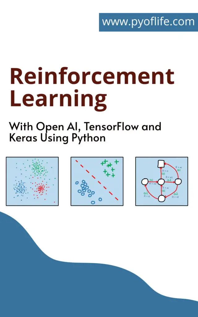
Reinforcement learning (RL) is a fascinating and rapidly evolving field within machine learning. By enabling agents to learn through interaction with their environment, RL has given rise to advancements in areas such as game playing, robotics, and autonomous systems. This article provides an in-depth look at reinforcement learning using OpenAI, TensorFlow, and Keras with Python. We’ll cover the fundamentals, delve into advanced techniques, and explore practical applications.
Introduction to Reinforcement Learning
Definition
Reinforcement learning is a subset of machine learning where an agent learns to make decisions by performing certain actions and observing the rewards/results of those actions. Unlike supervised learning, where the agent is provided with the correct answers during training, reinforcement learning involves learning through trial and error.
Importance
Reinforcement learning has significant implications for various fields, including robotics, game development, finance, healthcare, and more. It provides a framework for building intelligent systems that can adapt and improve over time without human intervention.
Applications
Game Playing: AlphaGo, developed by DeepMind, used RL to defeat the world champion Go player.
Robotics: Autonomous robots learn to navigate and perform tasks in dynamic environments.
Finance: RL algorithms optimize trading strategies and portfolio management.
Healthcare: Personalized treatment plans and drug discovery benefit from RL approaches.
Policy: A strategy used by the agent to decide actions based on the current state.
Value Function: A prediction of future rewards.
Q-Value (Action-Value): A value for action taken in a specific state.
Discount Factor (Gamma): Determines the importance of future rewards.
Theories
Markov Decision Process (MDP): A mathematical framework for modeling decision-making.
Bellman Equation: A recursive definition for the value function, fundamental in RL.
Understanding Agents and Environments
Types of Agents
Passive Agents: Only learn the value function.
Active Agents: Learn both the value function and the policy.
Environments
Deterministic vs. Stochastic: Deterministic environments have predictable outcomes, while stochastic ones involve randomness.
Static vs. Dynamic: Static environments do not change with time, whereas dynamic environments evolve.
Interactions
The agent-environment interaction can be modeled as a loop:
The agent observes the current state.
It chooses an action based on its policy.
The environment transitions to a new state and provides a reward.
The agent updates its policy based on the reward and new state.
OpenAI Gym Overview
Introduction
OpenAI Gym is a toolkit for developing and comparing reinforcement learning algorithms. It provides a standardized set of environments and a common interface.
Installation
To install OpenAI Gym, use the following command:
pip install gym
Basic Usage
import gym

# Create an environment
env = gym.make('CartPole-v1')

# Reset the environment to start
state = env.reset()

# Run a step
next_state, reward, done, info = env.step(env.action_space.sample())
Setting Up TensorFlow for RL
Installation
To install TensorFlow, use the following command:
pip install tensorflow
Configuration
Ensure you have a compatible version of Python and required dependencies. Verify the installation by running:
import tensorflow as tf
print(tf.__version__)
Environment Setup
For optimal performance, configure TensorFlow to utilize GPU if available:
import tensorflow as tf

if tf.test.gpu_device_name():
    print('GPU found')
else:
    print("No GPU found")
Keras Basics for RL
Installation
Keras is integrated with TensorFlow 2.x. You can install it along with TensorFlow:
pip install tensorflow
Key Features
Keras provides a high-level interface for building and training neural networks, simplifying the process of implementing deep learning models.
Basic Examples
import tensorflow as tf
from tensorflow.keras.models import Sequential
from tensorflow.keras.layers import Dense

# Define a simple model
model = Sequential([
    Dense(24, activation='relu', input_shape=(4,)),
    Dense(24, activation='relu'),
    Dense(2, activation='linear')
])

# Compile the model
model.compile(optimizer='adam', loss='mse')
Building Your First RL Model
Step-by-Step Guide Using OpenAI, TensorFlow, and Keras
Create the environment: Use OpenAI Gym to create the environment.
Define the model: Use Keras to build the neural network model.
Train the model: Implement the training loop using TensorFlow.
Evaluate the model: Test the model’s performance in the environment.
import gym
import tensorflow as tf
from tensorflow.keras.models import Sequential
from tensorflow.keras.layers import Dense
from tensorflow.keras.optimizers import Adam
import numpy as np

# Create the environment
env = gym.make('CartPole-v1')

# Define the model
model = Sequential([
    Dense(24, input_shape=(env.observation_space.shape[0],), activation='relu'),
    Dense(24, activation='relu'),
    Dense(env.action_space.n, activation='linear')
])

# Compile the model
model.compile(optimizer=Adam(learning_rate=0.001), loss='mse')

# Training loop
def train_model(env, model, episodes=1000):
    for e in range(episodes):
        state = env.reset()
        state = np.reshape(state, [1, env.observation_space.shape[0]])
        done = False
        while not done:
            action = np.argmax(model.predict(state))
            next_state, reward, done, _ = env.step(action)
            next_state = np.reshape(next_state, [1, env.observation_space.shape[0]])
            model.fit(state, reward, epochs=1, verbose=0)
            state = next_state
        print(f"Episode: {e+1}/{episodes}")

# Train the model
train_model(env, model)
Deep Q-Learning (DQN)
Theory
Deep Q-Learning is an extension of Q-Learning, where a neural network is used to approximate the Q-value function. It helps in dealing with large state spaces.
Implementation
import random

def deep_q_learning(env, model, episodes=1000, gamma=0.95, epsilon=1.0, epsilon_min=0.01, epsilon_decay=0.995):
    for e in range(episodes):
        state = env.reset()
        state = np.reshape(state, [1, env.observation_space.shape[0]])
        for time in range(500):
            if np.random.rand() <= epsilon:
                action = random.randrange(env.action_space.n)
            else:
                action = np.argmax(model.predict(state))
            next_state, reward, done, _ = env.step(action)
            reward = reward if not done else -10
            next_state = np.reshape(next_state, [1, env.observation_space.shape[0]])
            target = reward
            if not done:
                target = reward + gamma * np.amax(model.predict(next_state))
            target_f = model.predict(state)
            target_f[0][action] = target
            model.fit(state, target_f, epochs=1, verbose=0)
            state = next_state
            if done:
                print(f"Episode: {e+1}/{episodes}, score: {time}, epsilon: {epsilon:.2}")
                break
        if epsilon > epsilon_min:
            epsilon *= epsilon_decay

deep_q_learning(env, model)
Use Cases
Game Playing: DQN has been used to achieve human-level performance in Atari games.
Robotics: Autonomous robots use DQN for path planning and obstacle avoidance.
Policy Gradient Methods
Understanding Policy Gradients
Policy gradients directly optimize the policy by adjusting the parameters in the direction that increases the expected reward.
Implementation
import tensorflow as tf
from tensorflow.keras.models import Sequential
from tensorflow.keras.layers import Dense

# Define the policy network
policy_model = Sequential([
    Dense(24, activation='relu', input_shape=(4,)),
    Dense(24, activation='relu'),
    Dense(2, activation='softmax')
])

policy_model.compile(optimizer=Adam(learning_rate=0.01), loss='categorical_crossentropy')

def policy_gradient(env, model, episodes=1000):
    for e in range(episodes):
        state = env.reset()
        state = np.reshape(state, [1, env.observation_space.shape[0]])
        done = False
        rewards = []
        states = []
        actions = []
        while not done:
            action_prob = model.predict(state)
            action = np.random.choice(env.action_space.n, p=action_prob[0])
            next_state, reward, done, _ = env.step(action)
            states.append(state)
            actions.append(action)
            rewards.append(reward)
            state = np.reshape(next_state, [1, env.observation_space.shape[0]])
        discounted_rewards = discount_rewards(rewards)
        model.fit(np.vstack(states), np.vstack(actions), sample_weight=discounted_rewards, epochs=1, verbose=0)

def discount_rewards(rewards, gamma=0.99):
    discounted_rewards = np.zeros_like(rewards)
    cumulative = 0.0
    for t in reversed(range(len(rewards))):
        cumulative = cumulative * gamma + rewards[t]
        discounted_rewards[t] = cumulative
    return discounted_rewards

policy_gradient(env, policy_model)
Examples
Self-Driving Cars: Policy gradient methods help in developing policies for complex driving scenarios.
Financial Trading: Optimizing trading strategies by directly maximizing returns.
Actor-Critic Methods
Overview
Actor-Critic methods combine value-based and policy-based methods. The actor updates the policy, and the critic evaluates the action.
Advantages
Stability: Combines the advantages of value and policy-based methods.
Efficiency: More sample-efficient than pure policy gradient methods.
Implementation
from tensorflow.keras.models import Model
from tensorflow.keras.layers import Input, Dense
from tensorflow.keras.optimizers import Adam
import numpy as np

# Define actor-critic network
input_layer = Input(shape=(4,))
dense_layer = Dense(24, activation='relu')(input_layer)
dense_layer = Dense(24, activation='relu')(dense_layer)
action_output = Dense(2, activation='softmax')(dense_layer)
value_output = Dense(1, activation='linear')(dense_layer)

actor_critic_model = Model(inputs=input_layer, outputs=[action_output, value_output])
actor_critic_model.compile(optimizer=Adam(learning_rate=0.001), loss=['categorical_crossentropy', 'mse'])

def actor_critic(env, model, episodes=1000):
    for e in range(episodes):
        state = env.reset()
        state = np.reshape(state, [1, env.observation_space.shape[0]])
        done = False
        rewards = []
        states = []
        actions = []
        while not done:
            action_prob, value = model.predict(state)
            action = np.random.choice(env.action_space.n, p=action_prob[0])
            next_state, reward, done, _ = env.step(action)
            states.append(state)
            actions.append(action)
            rewards.append(reward)
            state = np.reshape(next_state, [1, env.observation_space.shape[0]])
        discounted_rewards = discount_rewards(rewards)
        advantages = discounted_rewards - np.vstack(model.predict(np.vstack(states))[1])
        model.fit(np.vstack(states), [np.vstack(actions), discounted_rewards], sample_weight=[advantages, advantages], epochs=1, verbose=0)

actor_critic(env, actor_critic_model)
Advanced RL Techniques
Double DQN
Double DQN addresses the overestimation bias in Q-learning by using two separate networks for action selection and evaluation.
Dueling DQN
Dueling DQN separates the estimation of the state value and the advantage of each action, providing more stable learning.
Prioritized Experience Replay
Prioritized experience replay improves learning efficiency by prioritizing more informative experiences for replay.
Implementation
Combining these techniques can be complex but significantly improves performance in challenging environments.
Using Neural Networks in RL
Architectures
Convolutional Neural Networks (CNNs): Used for processing visual inputs.
Recurrent Neural Networks (RNNs): Suitable for sequential data and environments with temporal dependencies.
Training
Training neural networks in RL involves using gradient descent to minimize the loss function, which can be complex due to the non-stationary nature of the environment.
Optimization
Gradient Clipping: Prevents exploding gradients.
Regularization: Techniques like dropout to prevent overfitting.
Hyperparameter Tuning in RL
Techniques
Grid Search: Exhaustively searching over a predefined set of hyperparameters.
Random Search: Randomly sampling hyperparameters from a distribution.
Bayesian Optimization: Using probabilistic models to find the best hyperparameters.
Tools
Optuna: An open-source hyperparameter optimization framework.
Hyperopt: A Python library for serial and parallel optimization over hyperparameters.
Best Practices
Start Simple: Begin with basic models and gradually increase complexity.
Use Validation Sets: Ensure that hyperparameter tuning is evaluated on a separate validation set.
Monitor Performance: Use metrics like reward, loss, and convergence time to guide tuning.
Exploration vs Exploitation
Balancing Strategies
Epsilon-Greedy: Start with high exploration (epsilon) and gradually reduce it.
Softmax: Select actions based on a probability distribution.
Methods
UCB (Upper Confidence Bound): Balances exploration and exploitation by considering both the average reward and uncertainty.
Thompson Sampling: Uses probability matching to balance exploration and exploitation.
Examples
Dynamic Environments: In scenarios where the environment changes over time, maintaining a balance between exploration and exploitation is crucial for continuous learning.
Reward Engineering
Designing Rewards
Sparse Rewards: Rewards given only at the end of an episode.
Dense Rewards: Frequent rewards to guide the agent’s behavior.
Shaping
Reward shaping involves modifying the reward function to provide intermediate rewards, helping the agent learn more effectively.
Use Cases
Robotics: Designing rewards for tasks like object manipulation or navigation.
Healthcare: Shaping rewards to optimize treatment plans.
RL in Robotics
Applications
Autonomous Navigation: Robots learn to navigate complex environments.
Manipulation: Robots learn to interact with and manipulate objects.
Industrial Automation: Optimizing processes and workflows in manufacturing.
Challenges
Safety: Ensuring safe interactions in dynamic environments.
Generalization: Adapting learned policies to new, unseen scenarios.
Case Studies
Boston Dynamics: Using RL for advanced robot locomotion.
OpenAI Robotics: Simulated and real-world robotic tasks using RL.
RL in Game Playing
Famous Examples
AlphaGo: Defeated the world champion Go player using deep RL.
Dota 2: OpenAI’s bots played and won against professional Dota 2 players.
Implementations
Monte Carlo Tree Search (MCTS): Combined with deep learning for strategic game playing.
Self-Play: Agents train by playing against themselves, improving over time.
Results
Superhuman Performance: RL agents achieving performance levels surpassing human experts.
Multi-Agent RL
Concepts
Cooperation: Agents work together to achieve a common goal.
Competition: Agents compete against each other.
Algorithms
Centralized Training with Decentralized Execution: Agents are trained together but act independently.
Multi-Agent Q-Learning: Extensions of Q-learning for multiple agents.
Applications
Traffic Management: Optimizing traffic flow using cooperative RL agents.
Energy Systems: Managing and optimizing power grids.
RL in Autonomous Systems
Self-Driving Cars
RL is used to develop driving policies, optimize routes, and enhance safety.
Drones
Autonomous drones use RL for navigation, obstacle avoidance, and mission planning.
Industrial Applications
Supply Chain Optimization: Using RL to improve efficiency and reduce costs.
Robotic Process Automation (RPA): Automating repetitive tasks using RL.
Evaluating RL Models
Metrics
Total Reward: Sum of rewards received by the agent.
Episode Length: Number of steps taken in an episode.
Success Rate: Proportion of episodes where the agent achieves its goal.
Tools
TensorBoard: Visualization tool for monitoring training progress.
Gym Wrappers: Custom wrappers to track and log performance metrics.
Techniques
Cross-Validation: Evaluating the model on multiple environments.
A/B Testing: Comparing different models or policies.
Common Challenges in RL
Overfitting
Overfitting occurs when the agent performs well in training but poorly in new environments. Mitigation strategies include using regularization techniques and ensuring a diverse training set.
Sample Efficiency
Sample efficiency refers to the number of interactions needed for the agent to learn. Techniques like experience replay and using model-based approaches can improve sample efficiency.
Scalability
Scaling RL algorithms to work with complex environments and large state spaces is challenging. Distributed RL and parallel training are common approaches to address this issue.
Debugging RL Models
Techniques
Logging: Keep detailed logs of training episodes, rewards, and losses.
Visualization: Use tools like TensorBoard to visualize training progress and identify issues.
Tools
Debugger: Python debuggers like pdb can help in step-by-step code execution.
Profiling: Use profiling tools to identify performance bottlenecks.
Best Practices
Start Simple: Begin with simple environments and gradually increase complexity.
Iterative Development: Implement and test in small increments to catch issues early.
Case Studies of RL
Success Stories
AlphaGo: Achieved superhuman performance in the game of Go.
OpenAI Five: Defeated professional Dota 2 players using multi-agent RL.
Failures
Tesla’s Autopilot: Early versions faced challenges with unexpected scenarios.
Google Flu Trends: Initially successful but later faced issues with prediction accuracy.
Lessons Learned
Iterative Improvement: Continuously improve models and policies based on feedback.
Robust Testing: Test extensively in diverse environments to ensure generalization.
Future of RL
Trends
Hybrid Approaches: Combining RL with other machine learning techniques.
Meta-RL: Developing agents that can learn how to learn.
AI Safety: Ensuring safe and ethical deployment of RL systems.
Predictions
Mainstream Adoption: RL will become more prevalent in various industries.
Improved Algorithms: Advances in algorithms will lead to more efficient and effective RL solutions.
Emerging Technologies
Quantum RL: Exploring the use of quantum computing in RL.
Neuromorphic Computing: Using brain-inspired computing for RL applications.
Ethics in RL
Ethical Considerations
Bias and Fairness: Ensuring RL systems do not reinforce biases.
Transparency: Making RL algorithms transparent and understandable.
Bias
Addressing bias in RL involves using fair data and ensuring diverse representation in training environments.
Fairness
Fairness in RL ensures that the benefits and impacts of RL systems are distributed equitably.
RL Research Directions
Open Problems
Exploration: Efficiently exploring large and complex state spaces.
Sample Efficiency: Reducing the number of interactions needed for effective learning.
Research Papers
“Human-Level Control Through Deep Reinforcement Learning” by Mnih et al.: A seminal paper on deep Q-learning.
“Proximal Policy Optimization Algorithms” by Schulman et al.: Introduced PPO, a popular RL algorithm.
Collaborations
Collaborations between academia, industry, and research institutions are essential for advancing RL.
Community and Resources for RL
Forums
Reddit: r/reinforcementlearning
Stack Overflow: RL tag for asking questions and finding solutions.
Blogs
OpenAI Blog: Insights and updates on RL research.
DeepMind Blog: Detailed posts on RL advancements and applications.
Conferences
NeurIPS: The Conference on Neural Information Processing Systems.
ICML: International Conference on Machine Learning.
Courses
Coursera: “Deep Learning Specialization” by Andrew Ng.
Reinforcement learning with OpenAI, TensorFlow, and Keras using Python offers a powerful approach to developing intelligent systems capable of learning and adapting. By understanding the fundamentals, exploring advanced techniques, and applying them to real-world scenarios, you can harness the potential of RL to solve complex problems and innovate in various fields. The future of RL is promising, with continuous advancements and growing applications across industries. Embrace this exciting journey and contribute to the evolution of intelligent systems.
Statistical analysis of financial data is crucial for making informed decisions in the finance industry. Using R, a powerful statistical programming language, can significantly enhance the accuracy and efficiency of your analysis. This article provides a comprehensive guide on how to perform statistical analysis of financial data using R.
R and RStudio are essential tools for statistical analysis. R is a programming language and software environment for statistical computing, while RStudio is an integrated development environment (IDE) for R.
Install R: Download and install R from the CRAN website.
Install RStudio: Download and install RStudio from the RStudio website.
Basics of R Programming
Understanding the basics of R programming is fundamental for performing statistical analysis. Here are a few key concepts:
Vectors and Data Frames: Vectors are the simplest data structures in R, while data frames are used to store tabular data.
Functions and Packages: R has numerous built-in functions and packages that extend its capabilities.
Data Manipulation: Techniques for data manipulation include subsetting, merging, and reshaping data.
“Quantitative Financial Analytics” by Edward M. Miller
Online Courses
“Financial Engineering and Risk Management” by Columbia University on Coursera
“Introduction to Computational Finance and Financial Econometrics” by the University of Washington on Coursera
Academic Papers
Access academic papers through databases like JSTOR and SSRN.
Conclusion
The statistical analysis of financial data in R is a powerful approach to understanding and interpreting complex financial datasets. By leveraging the extensive capabilities of R, financial analysts can perform robust analyses, make informed decisions, and manage risks effectively.
Practical Machine Learning with Python: Machine learning (ML) has transformed from a niche area of computer science to a mainstream technology with applications across various industries. From healthcare to finance, ML is driving innovation and providing solutions to complex problems. This guide aims to equip you with the practical skills and knowledge needed to build real-world intelligent systems using Python.
Understanding Machine Learning Basics
Machine learning is a subset of artificial intelligence that involves the development of algorithms that allow computers to learn from and make decisions based on data. There are three main types of machine learning:
Supervised Learning: Algorithms learn from labeled data and make predictions based on it.
Unsupervised Learning: Algorithms identify patterns and relationships in unlabeled data.
Reinforcement Learning: Algorithms learn by interacting with an environment and receiving feedback.
Why Python for Machine Learning?
Python has become the go-to language for machine learning due to its simplicity, versatility, and extensive library support. Some advantages of using Python include:
Ease of Use: Python’s syntax is straightforward and easy to learn.
Extensive Libraries: Libraries such as Scikit-Learn, TensorFlow, and Keras simplify the implementation of ML algorithms.
Community Support: A large and active community ensures a wealth of resources and continuous improvement.
Before diving into machine learning, it’s essential to set up your Python environment. This includes installing Python, choosing an Integrated Development Environment (IDE), and installing necessary packages:
Python Installation: Download and install the latest version of Python from the official website.
IDEs: Popular IDEs include Jupyter Notebook, PyCharm, and VSCode.
Packages: Install packages like NumPy, Pandas, and Matplotlib using pip.
Data Collection and Preprocessing
Data is the backbone of any machine learning project. The steps involved in data collection and preprocessing include:
Data Sources: Identify and gather data from reliable sources.
Data Cleaning: Handle missing values, remove duplicates, and correct errors.
Data Transformation: Normalize and scale data, encode categorical variables.
Exploratory Data Analysis (EDA)
EDA is a crucial step to understand the data and uncover insights. This involves:
Visualization: Use libraries like Matplotlib and Seaborn to create visual representations of data.
Insights: Identify patterns, trends, and anomalies.
Tools: Leverage tools like Pandas for data manipulation and analysis.
Feature Engineering
Feature engineering is the process of creating new features from raw data to improve model performance. Techniques include:
Feature Creation: Derive new features from existing ones.
Feature Selection: Identify and select the most relevant features.
Best Practices: Ensure features are relevant and avoid overfitting.
Supervised Learning
Supervised learning involves training models on labeled data to make predictions. Key algorithms include:
Regression: Predict continuous outcomes (e.g., house prices).
Predictions: Increased automation, enhanced model interpretability
Conclusion: Practical Machine Learning with Python
Machine learning with Python provides a powerful toolkit for solving real-world problems. By following this guide, you can build, evaluate, and deploy intelligent systems effectively. Stay updated with the latest trends and continue practicing to enhance your skills.
An Introduction to Spatial Data Analysis and Visualization in R: Spatial data analysis and visualization have become increasingly important in a variety of fields, ranging from environmental science and urban planning to epidemiology and marketing. Understanding the geographic patterns and relationships within data can provide valuable insights that inform decision-making and policy development. R, a powerful and versatile programming language, offers an extensive array of tools and packages designed specifically for spatial data analysis and visualization. This article serves as an introduction to these capabilities, providing a foundation for leveraging R in your spatial data projects.
What is Spatial Data?
Spatial data, also known as geospatial data, refers to information that has a geographic component. This type of data is associated with specific locations on the Earth’s surface and can be represented in various forms, such as points, lines, polygons, and rasters. Examples of spatial data include coordinates of landmarks, boundaries of administrative regions, routes of transportation networks, and satellite imagery.
Spatial data can be categorized into two main types:
Vector Data: Represents geographic features using points, lines, and polygons. Points can denote specific locations, lines can represent linear features like roads or rivers, and polygons can depict areas such as lakes or city boundaries.
Raster Data: Consists of a grid of cells or pixels, each with a value representing a specific attribute. Common examples include digital elevation models (DEMs) and remote sensing imagery.
Why Use R for Spatial Data Analysis and Visualization?
R is a highly regarded tool in the realm of data science due to its robust statistical analysis capabilities and extensive ecosystem of packages. When it comes to spatial data, R offers several advantages:
Comprehensive Package Ecosystem: R has numerous packages tailored for spatial data, including sf (simple features), sp, raster, and tmap. These packages provide tools for data manipulation, analysis, and visualization.
Integration with GIS: R can easily integrate with Geographic Information Systems (GIS) software, allowing for seamless data exchange and enhancing the analysis workflow.
Reproducibility: R scripts can be documented and shared, ensuring that analyses are reproducible and transparent.
Visualization Capabilities: R excels in data visualization, enabling the creation of detailed and customizable maps and plots.
Getting Started with Spatial Data in R
To begin working with spatial data in R, you’ll need to install and load several key packages. The sf package, which provides support for simple features, is widely used for handling vector data. For raster data, the raster package is essential. Here’s how to get started:
Vector data can be read into R using the st_read() function from the sf package. This function supports various file formats, including shapefiles and GeoJSON.
# Read a shapefile
shapefile_path <- "path/to/your/shapefile.shp"
vector_data <- st_read(shapefile_path)
Once loaded, you can manipulate the data using functions from the dplyr package, which integrates seamlessly with sf objects.
# Example of data manipulation
library(dplyr)
filtered_data <- vector_data %>%
  filter(attribute == "desired_value")
Loading and Manipulating Raster Data
Raster data can be read using the raster() function from the raster package.
Visualization is a critical aspect of spatial data analysis. The tmap package offers a flexible approach to creating static and interactive maps.
# Basic map of vector data
tm_shape(vector_data) +
  tm_borders() +
  tm_fill()

# Basic map of raster data
tm_shape(raster_data) +
  tm_raster()
The ggplot2 package, along with the geom_sf() function, can also be used for creating detailed and aesthetically pleasing maps.
library(ggplot2)
# Plot vector data with ggplot2
ggplot(data = vector_data) +
  geom_sf() +
  theme_minimal()
Conclusion
R provides a comprehensive suite of tools for spatial data analysis and visualization, making it a valuable asset for researchers, analysts, and professionals across various disciplines. By harnessing the power of R’s spatial packages, you can uncover geographic patterns, make informed decisions, and effectively communicate your findings through compelling visualizations. Whether you’re new to spatial data or looking to enhance your existing skills, mastering these tools will undoubtedly expand your analytical capabilities and open up new avenues for exploration and discovery.
Statistics and Machine Learning in Python: Python has rapidly become the go-to language for data science, largely due to its simplicity and the extensive range of libraries tailored for statistical analysis and machine learning. This guide delves into the essential tools and techniques for leveraging Python in these domains, providing a foundation for both beginners and seasoned professionals.
Understanding the Basics: Python for Data Science
Before diving into the specifics of statistics and machine learning, it’s crucial to understand why Python is so popular in data science:
Ease of Use: Python’s readable syntax and extensive documentation make it accessible for beginners.
Community Support: A large community means abundant resources, tutorials, and libraries.
Versatile Libraries: Python boasts libraries like NumPy, Pandas, Matplotlib, and SciPy that simplify data manipulation and visualization.
Core Libraries for Statistics
NumPy: Fundamental for numerical computations. It offers support for large multi-dimensional arrays and matrices, along with a collection of mathematical functions to operate on these arrays.
import numpy as np
data = np.array([1, 2, 3, 4, 5])
mean = np.mean(data)
print(mean)
Pandas: Essential for data manipulation and analysis. Pandas provide data structures like DataFrames, which are crucial for handling structured data.
Statsmodels: Provides classes and functions for the estimation of many different statistical models, including linear regression, time series analysis, and more.
import statsmodels.api as sm
X = df['column1']
y = df['column2']
X = sm.add_constant(X)  # Adds a constant term to the predictor
model = sm.OLS(y, X).fit()
predictions = model.predict(X)
print(model.summary())
Machine learning in Python is greatly facilitated by powerful libraries that allow for the implementation of complex algorithms with minimal code.
Scikit-Learn: The cornerstone for machine learning in Python. It provides simple and efficient tools for data mining and data analysis.
from sklearn.model_selection import train_test_split
from sklearn.linear_model import LinearRegression

X = df[['column1']]
y = df['column2']

X_train, X_test, y_train, y_test = train_test_split(X, y, test_size=0.2, random_state=0)
model = LinearRegression()
model.fit(X_train, y_train)
predictions = model.predict(X_test)
print(predictions)
TensorFlow and Keras: Used for building and training deep learning models. TensorFlow provides a flexible platform, while Keras offers a user-friendly interface.
import tensorflow as tf
from tensorflow.keras.models import Sequential
from tensorflow.keras.layers import Dense

model = Sequential()
model.add(Dense(10, input_dim=1, activation='relu'))
model.add(Dense(1))

model.compile(optimizer='adam', loss='mean_squared_error')
model.fit(X_train, y_train, epochs=50, batch_size=10)
predictions = model.predict(X_test)
print(predictions)
PyTorch: Another popular deep learning framework, known for its dynamic computation graph and ease of use, especially in research settings.
import torch
import torch.nn as nn
import torch.optim as optim

class SimpleModel(nn.Module):
    def __init__(self):
        super(SimpleModel, self).__init__()
        self.linear = nn.Linear(1, 1)

    def forward(self, x):
        return self.linear(x)

model = SimpleModel()
criterion = nn.MSELoss()
optimizer = optim.SGD(model.parameters(), lr=0.01)

for epoch in range(100):
    model.train()
    optimizer.zero_grad()
    outputs = model(torch.tensor(X_train, dtype=torch.float32))
    loss = criterion(outputs, torch.tensor(y_train, dtype=torch.float32))
    loss.backward()
    optimizer.step()

model.eval()
predictions = model(torch.tensor(X_test, dtype=torch.float32)).detach().numpy()
print(predictions)
Practical Applications and Projects
To solidify your understanding and gain practical experience, consider working on real-world projects such as:
Predictive Modeling: Build models to predict housing prices, stock market trends, or customer behavior.
Classification Tasks: Develop classifiers for email spam detection, image recognition, or disease diagnosis.
Natural Language Processing (NLP): Create applications for sentiment analysis, text generation, or machine translation.
Conclusion
Mastering statistics and machine learning in Python opens up a myriad of opportunities in data science and artificial intelligence. By leveraging Python’s powerful libraries and tools, you can efficiently analyze data, build predictive models, and derive insights that drive decision-making. Whether you’re a novice or an expert, Python’s ecosystem supports your journey through the fascinating world of data science.
Exploring Panel Data Econometrics with R: In the evolving landscape of econometrics, R is steadily gaining prominence. While traditionally overshadowed by other statistical software in econometrics, R’s popularity is rising due to its versatility and the development of specialized packages. “Panel Data Econometrics with R” by Yves Croissant and Giovanni Millo serves as a comprehensive guide for those looking to leverage R for panel data analysis.
Why R for Econometrics?
Econometrics is a field that demands rigorous model assumptions and extensive testing. R’s extensive suite of packages addresses these needs, offering tools for structural equation modeling, time series analysis, and robust covariance estimation, among others. The book highlights R’s edge in econometrics, emphasizing its open-source nature, extensive user community, and the ability to replicate and extend analyses easily .
Comprehensive Coverage: The book provides a thorough overview of basic to advanced econometric methods for panel data. It covers the essentials such as fixed effects, random effects, and mixed models, ensuring readers gain a solid foundation in the principles of panel data analysis .
Practical Examples: Staying true to R’s ethos of reproducibility, each chapter includes detailed examples with code that can be replicated by readers. This hands-on approach is beneficial for both students and practitioners, making complex concepts more accessible through practical application .
User-Centric Approach: The book is structured to cater to different levels of R users, from beginners to advanced programmers. It introduces the plm package for panel data analysis, guiding users through its functionalities and showing how it can be employed for various econometric tasks .
Extensive Resources: A companion package, pder, and additional resources are available online, enhancing the learning experience. These resources include datasets and code examples that complement the book’s content, making it easier for users to apply what they’ve learned to their own data .
Community and Development: The development of econometric tools in R is a collaborative effort. The book acknowledges contributions from various developers and the broader user community, showcasing the dynamic and supportive ecosystem surrounding R. This collaborative spirit is reflected in the continuous improvement and extension of R’s econometric capabilities .
Conclusion
“ExploringPanel Data Econometrics with R” is a valuable resource for anyone looking to delve into econometrics using R. It combines theoretical foundations with practical applications, making it a versatile tool for students, researchers, and practitioners alike. As R continues to grow in popularity within the econometric community, this book stands out as a key resource for harnessing its full potential in panel data analysis.
For those eager to explore the intersection of R and econometrics, this book offers a gateway to advanced analytical techniques, fostering a deeper understanding and application of econometric methods in various fields.
Machine learning has revolutionized numerous industries by enabling predictive analytics, which can anticipate trends, understand patterns, and make data-driven decisions. Python, with its robust libraries and ease of use, has become the go-to language for implementing machine learning algorithms. In this article, we’ll delve into essential techniques for predictive analysis using Python, providing a foundation for anyone looking to harness the power of machine learning.
Understanding Predictive Analysis
Predictive analysis involves using statistical algorithms and machine learning techniques to identify the likelihood of future outcomes based on historical data. It is a crucial aspect of business intelligence, aiding in everything from customer segmentation to risk management. The core components of predictive analysis include data preprocessing, model selection, training, evaluation, and deployment.
Data Preprocessing: Cleaning and Preparing Data
The first step in any machine learning project is data preprocessing. This involves cleaning and preparing the data to ensure that the machine learning model can learn effectively. Key tasks include handling missing values, removing duplicates, and encoding categorical variables.
Machine Learning in Python Essential Techniques for Predictive Analysis
Handling Missing Values: In Python, libraries such as Pandas make it straightforward to handle missing data. Techniques include imputation, where missing values are replaced with the mean, median, or mode of the column, or more advanced methods like using algorithms to predict missing values.
import pandas as pd
df = pd.read_csv('data.csv')
df.fillna(df.mean(), inplace=True)
Encoding Categorical Variables: Machine learning models require numerical input, so categorical data needs to be converted into a numerical format. This can be done using one-hot encoding or label encoding.
from sklearn.preprocessing import OneHotEncoder
encoder = OneHotEncoder()
df_encoded = encoder.fit_transform(df[['category']])
Feature Selection and Engineering
Feature selection involves identifying the most important variables that influence the outcome. Feature engineering, on the other hand, involves creating new features from existing data to improve model performance.
Feature Selection: Techniques like correlation matrices and recursive feature elimination (RFE) help in selecting relevant features.
from sklearn.feature_selection import RFE
from sklearn.linear_model import LogisticRegression
model = LogisticRegression()
rfe = RFE(model, 10)
fit = rfe.fit(X, y)
Feature Engineering: This involves creating new variables that might better capture the underlying patterns in the data. For example, creating interaction terms or polynomial features.
from sklearn.preprocessing import PolynomialFeatures
poly = PolynomialFeatures(degree=2)
X_poly = poly.fit_transform(X)
Model Selection: Choosing the Right Algorithm
Choosing the right machine learning algorithm is crucial for effective predictive analysis. Python offers a variety of algorithms through libraries like scikit-learn, TensorFlow, and PyTorch.
Linear Regression: Ideal for predicting continuous outcomes.
from sklearn.linear_model import LinearRegression
model = LinearRegression()
model.fit(X_train, y_train)
Decision Trees and Random Forests: Useful for both classification and regression tasks, these models are easy to interpret and can handle complex datasets.
from sklearn.ensemble import RandomForestClassifier
model = RandomForestClassifier()
model.fit(X_train, y_train)
Neural Networks: Powerful for capturing complex patterns in data, particularly with large datasets. Libraries like TensorFlow and Keras make it easier to build and train neural networks.
import tensorflow as tf
from tensorflow.keras.models import Sequential
from tensorflow.keras.layers import Dense
model = Sequential([
Dense(64, activation='relu', input_shape=(X_train.shape[1],)),
Dense(64, activation='relu'),
Dense(1, activation='sigmoid')
])
model.compile(optimizer='adam', loss='binary_crossentropy', metrics=['accuracy'])
model.fit(X_train, y_train, epochs=10)
Model Evaluation: Assessing Performance
Evaluating the performance of a machine learning model is critical to ensure its reliability and effectiveness. Common metrics include accuracy, precision, recall, F1 score, and ROC-AUC for classification tasks, and mean squared error (MSE) or R-squared for regression tasks.
Cross-Validation: A robust technique to ensure that the model generalizes well to unseen data.
from sklearn.model_selection import cross_val_score
scores = cross_val_score(model, X, y, cv=5)
Confusion Matrix and Classification Report: Provide detailed insights into the model’s performance.
Once the model is trained and evaluated, the final step is deployment. This involves integrating the model into a production environment where it can provide predictions on new data.
Saving the Model: Using libraries like joblib or pickle to save the trained model.
import joblib
joblib.dump(model, 'model.pkl')
API Integration: Deploying the model as a web service using frameworks like Flask or Django to provide real-time predictions.
from flask import Flask, request, jsonify
import joblib
app = Flask(name)
model = joblib.load('model.pkl')
@app.route('/predict', methods=['POST'])
def predict():
data = request.get_json()
prediction = model.predict(data['input'])
return jsonify({'prediction': prediction.tolist()})
if name == 'main':
app.run(debug=True)
Conclusion
Machine learning in Python is a powerful tool for predictive analysis, offering numerous libraries and techniques to build effective models. From data preprocessing to model deployment, understanding these essential techniques allows you to leverage machine learning to uncover valuable insights and make informed decisions. Whether you’re a beginner or an experienced data scientist, Python provides the flexibility and scalability to tackle predictive analytics projects of any complexity.
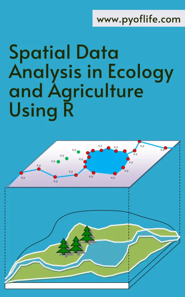
Spatial data analysis has become an essential tool in the fields of ecology and agriculture, enabling researchers and practitioners to understand and manage the spatial dynamics of various ecological and agricultural phenomena. With the advent of sophisticated software and programming languages, such as R, the capabilities for spatial data analysis have expanded significantly. This article explores the importance of spatial data analysis in these fields and how R facilitates this complex yet rewarding endeavor.
The Importance of Spatial Data in Ecology and Agriculture
Spatial data, which includes information about the location and distribution of variables across a geographic area, is crucial for understanding patterns and processes in both ecology and agriculture. In ecology, spatial data can reveal insights into species distribution, habitat fragmentation, and ecosystem dynamics. For agriculture, spatial data is instrumental in precision farming, crop monitoring, and land-use planning.
Applications in Ecology
Species Distribution Modeling (SDM): Understanding where species are likely to occur based on environmental conditions and geographical constraints is fundamental for conservation planning and biodiversity management.
Habitat Suitability Analysis: Identifying areas that are most suitable for specific species helps in creating protected areas and managing wildlife habitats effectively.
Landscape Ecology: Examining the spatial arrangement of ecosystems and their interactions helps ecologists understand ecological processes at a broader scale, such as nutrient cycling and energy flows.
Applications in Agriculture
Precision Agriculture: By analyzing spatial data from soil samples, crop yields, and weather patterns, farmers can optimize planting, irrigation, and fertilization practices to maximize productivity and sustainability.
Crop Monitoring: Satellite imagery and drone technology, coupled with spatial data analysis, allow for real-time monitoring of crop health, enabling early detection of issues such as disease or pest infestations.
Land-Use Planning: Spatial data helps in making informed decisions about land allocation, ensuring that agricultural activities are sustainable and do not adversely affect the environment.
R, a language and environment for statistical computing and graphics, has become a popular choice for spatial data analysis due to its extensive package ecosystem, powerful visualization capabilities, and robust statistical functions. Here are some key features and packages in R that make it indispensable for spatial data analysis in ecology and agriculture.
Key Features of R
Comprehensive Package Ecosystem: R boasts a wide array of packages specifically designed for spatial data analysis, such as sp, raster, sf, and spatstat.
Data Visualization: With packages like ggplot2 and leaflet, R provides powerful tools for creating informative and interactive maps and plots.
Statistical Analysis: R’s strong statistical capabilities allow for sophisticated analyses such as spatial regression, kriging, and spatial autocorrelation.
Essential R Packages for Spatial Data Analysis
sp: One of the foundational packages for handling spatial data, sp provides classes and methods for spatial data types.
raster: This package is essential for working with raster data, which is crucial for analyzing satellite imagery and environmental data.
sf: The sf package offers a more modern approach to handling spatial data in R, providing simple features that are compatible with the standards used in GIS software.
spatstat: Used for spatial point pattern analysis, spatstat is invaluable for analyzing the distribution of points in space, such as plant locations or animal sightings.
Practical Steps for Spatial Data Analysis in R
1. Data Import and Preparation
The first step in spatial data analysis is importing and preparing the data. R can handle various data formats, including shapefiles, GeoTIFFs, and CSV files with spatial coordinates.
library(sf)
library(raster)

# Load a shapefile
shape_data <- st_read("path_to_shapefile.shp")

# Load a raster file
raster_data <- raster("path_to_raster.tif")
2. Data Visualization
Visualizing spatial data is crucial for understanding patterns and communicating results. R’s ggplot2 and leaflet packages are excellent for creating static and interactive maps.
library(ggplot2)
library(leaflet)

# Plot shapefile data with ggplot2
ggplot(data = shape_data) +
  geom_sf()

# Create an interactive map with leaflet
leaflet(shape_data) %>%
  addTiles() %>%
  addPolygons()
3. Spatial Analysis
Conducting spatial analysis involves using statistical techniques to analyze spatial data. For example, performing a kriging interpolation can predict values at unsampled locations.
Finally, interpreting the results and generating reports or publications is the last step. R’s rmarkdown package allows for seamless integration of analysis and reporting.
library(rmarkdown)

# Create a report
render("analysis_report.Rmd")
Conclusion
Spatial data analysis is a powerful approach that enhances our understanding and management of ecological and agricultural systems. R, with its extensive packages and capabilities, offers a robust platform for conducting spatial data analysis. By leveraging these tools, researchers and practitioners can make data-driven decisions that promote sustainability and conservation in these vital fields. Whether it’s predicting species distributions, optimizing crop yields, or planning land use, the integration of spatial data analysis with R is proving to be transformative.
Learning Python’s Basic Statistics with ChatGPT: Python has cemented its place as a preferred programming language for data analysis due to its ease of use and robust library ecosystem. Among its many capabilities, Python’s statistical functions stand out, allowing users to perform intricate data analyses effortlessly. This article explores how to leverage Python’s statistical tools with the assistance of ChatGPT, a powerful language model designed to facilitate learning and application of these tools.
Understanding Python’s Statistical Packages
Python offers a myriad of packages tailored for statistical analysis. Key libraries include:
NumPy: Essential for numerical computing, NumPy provides a powerful array object and numerous functions for array manipulation and statistical analysis.
Pandas: Ideal for data manipulation and analysis, Pandas introduces data structures like DataFrames to handle and analyze large datasets efficiently.
SciPy: Built for scientific computing, SciPy includes modules for optimization, integration, interpolation, and statistical analysis.
Statsmodels: This library focuses on statistical modeling, providing tools for regression analysis, time series analysis, and more.
These libraries collectively empower Python users to perform a wide range of statistical operations, from basic descriptive statistics to complex inferential tests.
The study conducted utilized ChatGPT to enhance the understanding and execution of statistical analyses in Python. By interacting with ChatGPT, users can obtain explanations, code snippets, and guidance on various statistical methods. Below are some insights derived from using ChatGPT:
Example Analyses Using Python
T-Test: A T-test helps determine if there is a significant difference between the means of two groups. Here’s a Python example using the scipy.stats library:
import numpy as np
from scipy.stats import ttest_ind

# Generate two sets of data
group1 = np.random.normal(5, 1, 100)
group2 = np.random.normal(7, 1, 100)

# Calculate the T-test
t_statistic, p_value = ttest_ind(group1, group2)

# Print the results
print("T-test statistic:", t_statistic)
print("P-value:", p_value)
This script generates two random datasets and performs a T-test to compare their means, providing both the T-statistic and p-value to evaluate significance.
Mann-Whitney U Test: Used when data doesn’t follow a normal distribution, the Mann-Whitney U test compares the medians of two independent groups. Here’s how to execute it in Python:
from scipy.stats import mannwhitneyu

# Define the two groups
group1 = [3, 4, 5, 6, 7, 8, 9]
group2 = [1, 2, 3, 4, 5]

# Perform the Mann-Whitney U test
statistic, p_value = mannwhitneyu(group1, group2, alternative='two-sided')

# Print the results
print("Mann-Whitney U statistic:", statistic)
print("p-value:", p_value)
This example illustrates comparing two groups’ medians and provides the U statistic and p-value for significance testing.
Visualizing Statistical Results
Visualization is crucial for interpreting statistical results. Python’s matplotlib and seaborn libraries are invaluable for creating informative visualizations. For instance, box plots and histograms can effectively display data distributions and test results.
Box Plot: A box plot compares the distributions of two groups, highlighting medians and quartiles.
import matplotlib.pyplot as plt
import seaborn as sns

# Define the two groups
group1 = [3, 4, 5, 6, 7, 8, 9]
group2 = [1, 2, 3, 4, 5]

# Create a box plot
sns.boxplot(x=['Group 1']*len(group1) + ['Group 2']*len(group2), y=group1+group2)

# Add titles and labels
plt.title('Box plot of two groups')
plt.xlabel('Group')
plt.ylabel('Value')

# Show the plot
plt.show()
Histogram: A histogram visualizes the frequency distribution of data points within each group.
# Create histograms of the two groups
sns.histplot(group1, kde=True, color='blue', alpha=0.5, label='Group 1')
sns.histplot(group2, kde=True, color='green', alpha=0.5, label='Group 2')

# Add titles and labels
plt.title('Histogram of two groups')
plt.xlabel('Value')
plt.ylabel('Frequency')

# Add a legend
plt.legend()

# Show the plot
plt.show()
These visual tools, combined with statistical tests, provide a comprehensive approach to data analysis, making the interpretation of results more intuitive.
Conclusion
Python’s statistical libraries, when used in conjunction with ChatGPT, offer a powerful toolkit for data analysis. By leveraging these resources, users can perform complex statistical tests, visualize their results effectively, and gain deeper insights into their data. Whether you’re a beginner or an experienced analyst, integrating ChatGPT with Python’s statistical capabilities can significantly enhance your analytical workflow.