SAROJ

Visualizing Climate Change Data with R

Visualizing Climate Change Data with R: Climate change is one of the most pressing global issues of our time, and effective communication of its impacts is essential. Data visualization plays a critical role in presenting complex climate data in an accessible and compelling way. For researchers, policymakers, and activists, R—a powerful programming language for statistical computing—offers extensive tools to create engaging visualizations. In this article, we’ll explore how you can leverage R to visualize climate change data effectively.

Why Visualize Climate Change Data?

Climate change data, such as temperature anomalies, CO2 emissions, and sea level rise, often involves large datasets and intricate patterns. Visualization helps:

  1. Simplify Complexity: Transform raw data into intuitive graphics.

  2. Highlight Trends: Spot patterns and changes over time.
  3. Engage Audiences: Communicate findings effectively to non-experts.
  4. Drive Action: Persuade stakeholders to take informed actions.

    Download (PDF)

Getting Started with R for Climate Data Visualization

R provides robust packages for data manipulation, analysis, and visualization. Here’s how you can begin:

1. Install Required Packages

Popular R packages for climate data visualization include:

  • ggplot2: A versatile package for creating static and interactive visualizations.
  • leaflet: Useful for interactive maps.
  • sf: For handling spatial data.
  • raster: Excellent for working with raster datasets like satellite imagery.
  • climdex.pcic: Designed specifically for climate indices.
install.packages(c("ggplot2", "leaflet", "sf", "raster", "climdex.pcic"))

2. Access Climate Data

You can source climate data from:

  • NASA: Global climate models and satellite observations.
  • NOAA: Historical weather and climate data.
  • IPCC: Reports and datasets on global warming.
  • World Bank: Open climate data for development projects.

3. Load and Clean Data

Climate datasets are often large and require preprocessing. Use libraries like dplyr and tidyr for data cleaning:

library(dplyr)
climate_data <- read.csv("temperature_anomalies.csv")
clean_data <- climate_data %>% filter(!is.na(Temperature))

Examples of Climate Data Visualizations in R

1. Line Plot for Temperature Trends

library(ggplot2)
ggplot(clean_data, aes(x = Year, y = Temperature)) +
geom_line(color = "red") +
labs(title = "Global Temperature Anomalies Over Time",
x = "Year",
y = "Temperature Anomaly (Celsius)") +
theme_minimal()


This plot shows the trend in global temperature anomalies, highlighting warming over decades.

2. Mapping CO2 Emissions

library(leaflet)
leaflet(data = co2_data) %>%
addTiles() %>%
addCircles(lng = ~Longitude, lat = ~Latitude, weight = 1,
radius = ~Emissions * 1000, popup = ~paste(Country, Emissions))


Interactive maps like this allow users to explore geographic patterns in emissions.

3. Visualizing Sea Level Rise with Raster Data

library(raster)
sea_level <- raster("sea_level_rise.tif")
plot(sea_level, main = "Projected Sea Level Rise", col = terrain.colors(10))


Raster visuals are ideal for showing spatial variations in sea level projections.

Tips for Effective Climate Data Visualization

  1. Know Your Audience: Tailor visuals for scientists, policymakers, or the public.
  2. Use Clear Labels: Ensure axis labels, legends, and titles are easy to understand.
  3. Choose the Right Chart: Use line graphs for trends, maps for spatial data, and bar charts for comparisons.
  4. Leverage Color: Use color to enhance clarity but avoid misleading representations.
  5. Encourage Interaction: Interactive visuals engage viewers and allow deeper exploration.

Conclusion

R is a powerful tool for visualizing climate change data, offering diverse packages and customization options to create impactful graphics. Whether you’re illustrating global temperature trends or mapping carbon emissions, effective visualizations can make your findings more accessible and actionable. Start leveraging R today to communicate climate change insights and drive meaningful change.

Download: Data Visualization In R with 100 Examples

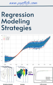
Regression Modeling Strategies

In today’s data-driven world, regression modeling has become a cornerstone of predictive analytics, enabling businesses and researchers to uncover insights and make data-backed decisions. Understanding regression modeling strategies is essential for building robust models, improving accuracy, and addressing real-world complexities.

This article dives into the core concepts, strategies, and best practices in regression modeling, tailored for both beginners and advanced practitioners.

What Is Regression Modeling?

Regression modeling is a statistical technique used to examine the relationship between a dependent variable and one or more independent variables. It predicts outcomes, identifies trends, and determines causal relationships in a variety of fields, including finance, healthcare, and marketing.

Popular types of regression models include:

Key Strategies in Regression Modeling

  1. Data Preparation and Exploration
    • Clean the Data: Handle missing values, outliers, and ensure data consistency.
    • Understand Relationships: Use visualization tools to explore variable relationships.

    Tip: Correlation matrices and scatterplots can help identify multicollinearity and initial patterns.

  2. Model Selection
    • Match the model to your problem. For example, use logistic regression for classification tasks and ridge regression to handle overfitting in high-dimensional data.
    • Leverage model evaluation metrics like R-squared, AIC, and BIC to compare performance.
  3. Feature Engineering
    • Create New Features: Combine or transform existing variables for improved predictive power.
    • Standardize or Normalize: Scale variables to ensure fair contributions to the model.
  4. Addressing Multicollinearity
    Multicollinearity occurs when independent variables are highly correlated, which can distort estimates. Address it through:

    • Dropping redundant variables.
    • Using regularization techniques like ridge or lasso regression.
  5. Validation and Testing
    • Split the data into training, validation, and testing sets.
    • Use cross-validation to ensure model generalizability.
  6. Interpretability
    • Keep the model understandable by minimizing unnecessary complexity.
    • Use tools like partial dependence plots and feature importance rankings to explain model behavior.

Advanced Techniques to Improve Regression Models

  • Regularization Methods: Employ ridge and lasso regression to shrink coefficients and enhance model stability.
  • Interaction Terms: Capture relationships between variables by including interaction effects in the model.
  • Non-linear Models: Use polynomial regression or generalized additive models (GAMs) for non-linear relationships.
  • Automated Model Tuning: Leverage tools like grid search or Bayesian optimization to fine-tune hyperparameters.

Applications of Regression Modeling

Regression modeling has versatile applications:

  • Healthcare: Predict patient outcomes or disease risks.
  • Marketing: Optimize campaign performance by analyzing customer data.
  • Finance: Forecast stock prices, credit risks, or economic trends.
  • Manufacturing: Predict equipment failures and optimize production processes.

Challenges and Best Practices

Despite its power, regression modeling comes with challenges:

  • Overfitting: Avoid models that perform well on training data but fail to generalize.
  • Data Quality: Poor data can lead to inaccurate predictions.
  • Bias-Variance Tradeoff: Balance model complexity to minimize prediction errors.

Best Practices:

  • Always validate your model on unseen data.
  • Regularly revisit the model as new data becomes available.
  • Document assumptions and ensure ethical use of data.

Conclusion

Regression modeling strategies provide a structured approach to uncovering meaningful patterns and making reliable predictions. By combining data preparation, thoughtful model selection, and rigorous testing, you can create robust models that drive actionable insights. Whether you’re solving business challenges or advancing research, mastering these strategies is essential for success.

Download: Linear Regression Using R: An Introduction to Data Modeling

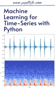
Machine Learning for Time-Series with Python

Machine Learning for Time-Series with Python: Machine Learning (ML) has revolutionized various industries, and its application in time-series analysis is no exception. Time-series data, characterized by observations collected at successive points in time, can unlock powerful insights when analyzed correctly. Python, with its robust libraries and frameworks, has become the go-to tool for time-series ML. In this article, we’ll explore how to leverage Python for time-series analysis, tools and techniques, and real-world applications.

What is Time-Series Data?

Time-series data represents information recorded at different time intervals. Common examples include stock prices, weather data, sensor readings, and economic indicators. These datasets often exhibit trends, seasonality, and noise, making them unique and challenging for machine learning models.

Why Use Machine Learning for Time-Series Analysis?

Traditional statistical methods like ARIMA and SARIMA are excellent for stationary time-series, but ML models bring versatility, scalability, and predictive accuracy to the table. With ML, you can:

  • Handle non-linear relationships.
  • Work with multivariate data.
  • Build robust models for forecasting, anomaly detection, and classification.

Key Python Libraries for Time-Series ML

Python boasts several powerful libraries for time-series analysis:

  1. Pandas: For data manipulation and preparation.
  2. NumPy: For numerical computations.
  3. Matplotlib & Seaborn: For data visualization.
  4. Statsmodels: For traditional time-series models like ARIMA.
  5. Scikit-learn: For machine learning models.
  6. TensorFlow & PyTorch: For deep learning models.
  7. TSFresh & Sktime: For feature extraction and time-series specific modeling.

    Download (PDF)

Steps to Perform Machine Learning on Time-Series Data

  1. Exploratory Data Analysis (EDA)
    • Visualize the data to understand trends, seasonality, and anomalies.
    • Use Pandas and Matplotlib for plotting and summary statistics.
  2. Data Preprocessing
    • Handle missing values using interpolation or forward-filling.
    • Resample data if needed (e.g., from hourly to daily observations).
    • Normalize or scale features for better model performance.
  3. Feature Engineering
    • Extract time-based features like day, month, year, or holiday indicators.
    • Create lag features and rolling statistics (e.g., moving averages).
    • Use libraries like TSFresh for automated feature extraction.
  4. Model Selection
    • For simple tasks: Use regression models like Random Forests or Gradient Boosting.
    • For sequence learning: Explore Recurrent Neural Networks (RNNs), LSTMs, or Transformers.
  5. Training and Evaluation
    • Split data into training and testing sets while preserving temporal order.
    • Evaluate models using metrics like RMSE, MAE, or MAPE.
  6. Forecasting
    • Use Sktime or deep learning libraries for robust forecasting capabilities.

Real-World Applications of Time-Series ML

  1. Finance: Stock price forecasting, risk analysis, and fraud detection.
  2. Healthcare: Monitoring patient vitals and disease progression.
  3. Retail: Demand forecasting and inventory management.
  4. IoT: Predictive maintenance using sensor data.
  5. Climate Science: Weather prediction and climate modeling.

Example: Forecasting with LSTM in Python

Here’s a snippet to forecast time-series data using LSTM in Python:

import numpy as np
import pandas as pd
from sklearn.preprocessing
import MinMaxScaler
from tensorflow.keras.models
import Sequential
from tensorflow.keras.layers import LSTM, Dense
# Load data
data = pd.read_csv('time_series_data.csv')
data_values = data['value'].values.reshape(-1, 1)
# Normalize data
scaler = MinMaxScaler()
data_scaled = scaler.fit_transform(data_values)
# Prepare sequences
def create_sequences(data, time_steps):
sequences = []
for i in range(len(data) - time_steps):
sequences.append((data[i:i + time_steps], data[i + time_steps]))
return np.array(sequences)
time_steps = 10
sequences = create_sequences(data_scaled, time_steps)
X, y = zip(*sequences)
X, y = np.array(X), np.array(y)
# Build LSTM model
model = Sequential([
LSTM(50, return_sequences=True, input_shape=(X.shape[1], X.shape[2])),
LSTM(50, return_sequences=False),
Dense(1)
])
model.compile(optimizer='adam', loss='mse')
model.fit(X, y, epochs=10, batch_size=32)
# Forecasting
predictions = model.predict(X)

Best Practices for Time-Series ML

  1. Ensure data integrity and quality.
  2. Avoid data leakage by splitting datasets carefully.
  3. Regularly validate model performance on unseen data.
  4. Consider domain-specific knowledge for feature engineering.

Conclusion

Machine learning has transformed time-series analysis by enabling more dynamic, accurate, and versatile models. With Python’s vast ecosystem of tools and libraries, analysts and developers can easily tackle challenges in time-series data. From forecasting stock prices to detecting anomalies in IoT, the possibilities are endless. Start exploring today and unlock the power of time-series with Python!

Download: Introduction to Time Series with Python

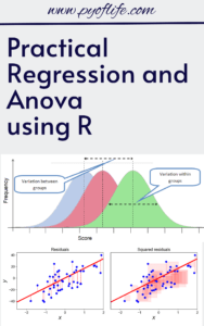
Practical Regression and Anova using R

Practical Regression and Anova using R: Regression analysis and Analysis of Variance (ANOVA) are foundational statistical tools used in research to understand relationships between variables and differences among groups. In this guide, we’ll walk through practical examples of these techniques using R, a popular statistical programming language. This article assumes a basic understanding of R and is structured to facilitate step-by-step learning.

Section 1: Linear Regression

1.1 Overview

Linear regression models the relationship between a dependent variable y and one or more independent variables x. The simplest form is simple linear regression, where one independent variable predicts y.

1.2 Performing Simple Linear Regression in R

Example:

Suppose you have a dataset mtcars and want to predict miles-per-gallon (mpg) using the weight of the car (wt).

# Load dataset
data(mtcars)
# Fit a simple linear regression model
model <- lm(mpg ~ wt, data = mtcars)# Summary of the model
summary(model)

Key Outputs:

  1. Coefficients: The intercept and slope tell us how mpg changes with wt.
  2. R-squared: Measures how well the model explains the variability in mpg.

Visualization:

# Scatter plot with regression line
plot(mtcars$wt, mtcars$mpg, main = "Weight vs MPG", xlab = "Weight", ylab = "MPG", pch = 19)
abline(model, col = "blue")

1.3 Multiple Linear Regression

Extend the model to include more predictors, e.g., hp (horsepower).

# Fit a multiple linear regression model
model_multi <- lm(mpg ~ wt + hp, data = mtcars)
# Summary of the model
summary(model_multi)

Interpretation:

Each coefficient represents the effect of a variable on mpg, holding other variables constant.

Practical Regression and Anova using R

Practical Regression and Anova using R

Download (PDF)

Section 2: Analysis of Variance (ANOVA)

2.1 Overview

ANOVA compares means across groups to determine if the differences are statistically significant.

One-Way ANOVA Example:

Does the average mpg differ across different numbers of cylinders (cyl) in mtcars?

# Fit a one-way ANOVA model
anova_model <- aov(mpg ~ factor(cyl), data = mtcars)
# Summary of the model
summary(anova_model)

Key Outputs:

  1. F-statistic: Indicates whether group means are significantly different.
  2. p-value: Determines the significance of the differences.

Visualization:

# Boxplot for visualization
boxplot(mpg ~ factor(cyl), data = mtcars, main = "MPG by Number of Cylinders", xlab = "Cylinders", ylab = "MPG")

2.2 Post-Hoc Testing

If ANOVA indicates significant differences, conduct post-hoc tests to identify which groups differ.

# Post-hoc test using Tukey's Honest Significant Differences
TukeyHSD(anova_model)

2.3 Two-Way ANOVA

Add another factor, e.g., interaction between cyl and gear.

# Two-way ANOVA
anova_model2 <- aov(mpg ~ factor(cyl) * factor(gear), data = mtcars)
# Summary
summary(anova_model2)

Section 3: Practical Tips

  1. Data Inspection:

    • Always inspect data for missing values and outliers.
    • Use summary()str(), and head() functions in R for exploration.
  2. Assumption Checking:

    • For regression: Check linearity, normality, and homoscedasticity.
    • For ANOVA: Check normality and equality of variances.
    •  plotUse diagnostics:
      par(mfrow = c(2, 2))
      plot(model)
  3. Model Refinement:
    • Simplify models by removing insignificant predictors using stepwise selection (step() function).

Conclusion

Regression and ANOVA are versatile tools for data analysis. R provides a robust platform with simple functions to execute these methods and generate visualizations. Practice is key—try these techniques on real datasets to gain proficiency.

For more resources, explore R’s built-in documentation (?lm?aov) and packages like car for advanced regression diagnostics.

Download: New Approach to Regression with R

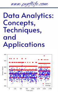
Data Analytics: Concepts, Techniques, and Applications

Data Analytics: Concepts, Techniques, and Applications: In today’s data-driven world, organizations of all sizes rely on data analytics to gain insights, improve decision-making, and drive innovation. Understanding the fundamentals of data analytics, the techniques involved, and its diverse applications can provide a competitive edge. This article explores these core aspects in depth.

What is Data Analytics?

Data analytics refers to the process of examining, cleaning, transforming, and modeling data to uncover meaningful patterns, trends, and insights. It combines statistical analysis, machine learning, and visualization tools to interpret data and support decision-making.

Key Concepts in Data Analytics

  1. Data Collection: Gathering relevant data from various sources such as databases, APIs, and sensors.

  2. Data Cleaning: Removing inaccuracies and inconsistencies to ensure data quality.
  3. Data Transformation: Converting raw data into a format suitable for analysis.
  4. Data Analysis: Using techniques like statistical modeling and machine learning to interpret data.
  5. Visualization: Presenting data insights in visual formats like charts and dashboards.

    Download (PDF)

Techniques in Data Analytics

A range of techniques is employed in data analytics to derive actionable insights:

1. Descriptive Analytics

This technique focuses on summarizing past data to understand historical trends. Methods include:

  • Data aggregation

  • Statistical summaries
  • Visualization tools

2. Predictive Analytics

Predictive analytics uses historical data and machine learning models to forecast future trends. Techniques include:

  • Regression analysis

  • Neural networks
  • Decision trees

3. Prescriptive Analytics

Prescriptive analytics recommends actions based on data insights. It combines predictive models with optimization algorithms.

4. Diagnostic Analytics

This method digs deeper into data to determine the reasons behind past outcomes. It uses:

  • Root cause analysis

  • Drill-down techniques
  • Correlation analysis

5. Real-Time Analytics

Real-time analytics processes data as it arrives, enabling immediate insights and responses. Common in industries like finance and e-commerce, it involves technologies like streaming analytics and edge computing.

Applications of Data Analytics

Data analytics has transformative applications across various industries:

1. Business

  • Customer Insights: Analyzing purchasing behaviors to enhance customer experiences.

  • Operations Management: Streamlining supply chains and reducing operational costs.

2. Healthcare

  • Patient Care: Predictive models for disease diagnosis and treatment.

  • Hospital Management: Improving resource allocation and reducing patient wait times.

3. Finance

  • Fraud Detection: Identifying anomalous transactions to prevent fraud.

  • Investment Analysis: Predicting market trends to inform investment strategies.

4. Retail

  • Personalized Marketing: Using customer data to tailor marketing campaigns.

  • Inventory Management: Optimizing stock levels based on sales trends.

5. Manufacturing

  • Predictive Maintenance: Monitoring equipment to predict and prevent failures.

  • Quality Control: Analyzing production data to ensure consistent quality.

6. Education

  • Learning Analytics: Tracking student performance to personalize learning experiences.

  • Administrative Efficiency: Enhancing resource planning and allocation.

7. Government

  • Policy Making: Using analytics to design data-driven policies.

  • Public Safety: Analyzing crime data to improve law enforcement strategies.

The Future of Data Analytics

With advancements in artificial intelligence, big data, and cloud computing, data analytics continues to evolve. Emerging trends include:

  • Augmented Analytics: Automating insights with AI and machine learning.

  • Edge Analytics: Performing analytics closer to the source of data generation.
  • Explainable AI: Enhancing transparency in complex predictive models.

Conclusion

Data analytics is an indispensable tool for modern organizations, offering powerful techniques and diverse applications to unlock the potential of data. By understanding its concepts, mastering its techniques, and exploring its applications, businesses and professionals can harness its full potential to drive growth and innovation.

Download: Advanced Data Analytics Using Python

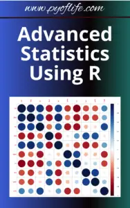
Mastering Advanced Statistics Using R

Statistics is the backbone of data-driven decision-making, and R has become the go-to tool for statisticians and data analysts worldwide. With its rich ecosystem of libraries and intuitive syntax, R simplifies complex statistical analysis and empowers users to extract actionable insights from data. This blog will walk you through the fundamentals and advanced features of R for statistics, ensuring you unlock the full potential of this powerful programming language.

Why Use R for Advanced Statistics?

R excels in statistical computing for several reasons:

  1. Specialized Libraries: Packages like dplyrggplot2caret, and MASS provide functionalities tailored to various statistical needs.
  2. Data Visualization: R offers state-of-the-art visualization tools that make your statistical findings easy to interpret and present.
  3. Community Support: A vibrant community ensures frequent updates, new packages, and a wealth of learning resources.
  4. Flexibility and Integration: R integrates seamlessly with Python, SQL, and big data tools like Hadoop and Spark.

    Download PDF

Key Features for Advanced Statistical Analysis

1. Linear and Non-linear Modeling

  • Linear Regression: The lm() function in R is a powerful tool for predicting relationships between variables.
  • Non-linear Models: R handles complex relationships using functions like nls() and packages like nlme.

Example:

model <- lm(y ~ x1 + x2, data = dataset)
summary(model)

2. Multivariate Analysis

Techniques like Principal Component Analysis (PCA) and Cluster Analysis can be implemented easily using libraries like stats and FactoMineR.

  • PCA: Dimensionality reduction to simplify datasets.
  • Cluster Analysis: Grouping similar observations for pattern recognition.

3. Time-Series Analysis

R’s forecast and tsibble packages are tailored for analyzing and predicting trends over time.
Example:

library(forecast)
fit <- auto.arima(time_series_data)
forecast(fit, h = 10)

4. Bayesian Statistics

R integrates Bayesian methods through packages like rstan and bayesplot. These tools allow you to perform probabilistic modeling and inference.

5. Machine Learning Integration

With packages like caret and mlr, you can blend statistical analysis with machine learning techniques, from decision trees to ensemble methods.

How to Get Started with R for Advanced Statistics?

Step 1: Install Essential Libraries

Start by installing foundational libraries:

install.packages(c("dplyr", "ggplot2", "caret", "MASS"))

Step 2: Understand Your Data

Explore your dataset with summary statistics and visualizations:

summary(dataset)
plot(dataset$x, dataset$y)

Step 3: Apply Advanced Methods

Dive into specific statistical techniques that match your project needs, from regression to hypothesis testing.

Tips for Mastering R for Advanced Statistics

  1. Leverage Online Resources: Use platforms like CRAN, Stack Overflow, and R-bloggers for learning.
  2. Practice Regularly: Build projects, analyze real-world datasets, and replicate case studies to sharpen your skills.
  3. Focus on Visualization: Master ggplot2 to create compelling visual narratives for your analyses.

Conclusion

Advanced statistics using R opens up endless possibilities for data exploration, modeling, and prediction. Whether you’re analyzing large datasets or diving deep into Bayesian methods, R equips you with the tools needed for success. Start today, and transform your data into impactful insights.

Download: Applied Statistics: Theory and Problem Solutions with R

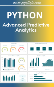
Python: Advanced Predictive Analytics

Predictive analytics has revolutionized the way businesses make decisions, allowing them to anticipate future trends, identify risks, and seize opportunities with precision. Python, with its rich ecosystem of libraries and tools, is at the forefront of this transformation. In this blog, we’ll explore how Python empowers professionals to excel in advanced predictive analytics and unlock new potential in data-driven decision-making.

Why Python for Predictive Analytics?

Python has emerged as the go-to programming language for predictive analytics due to its simplicity, versatility, and robust libraries. Key features include:

  • Rich Library Ecosystem: Libraries like Pandas, NumPy, and SciPy simplify data manipulation and mathematical computations, while tools like Scikit-learn, TensorFlow, and PyTorch enable machine learning and deep learning capabilities.
  • Visualization Powerhouses: Tools like Matplotlib, Seaborn, and Plotly allow for insightful and interactive data visualization.
  • Scalability and Integration: Python easily integrates with databases, APIs, and big data platforms, making it highly scalable for enterprise-level analytics.

    Download (PDF)

Key Techniques in Advanced Predictive Analytics with Python

1. Time Series Forecasting

Time series analysis is vital for predicting trends like stock prices, sales, and weather patterns. Python’s statsmodels and prophet libraries excel at implementing ARIMA, SARIMA, and advanced models for precise forecasting.

Example: Using Facebook’s Prophet library for predicting sales trends:

from fbprophet import Prophet
import pandas as pd

data = pd.read_csv('sales_data.csv')

model = Prophet()
model.fit(data)
forecast = model.predict(future)

2. Machine Learning for Predictive Modeling

Python’s Scikit-learn provides algorithms like decision trees, random forests, and gradient boosting for classification and regression tasks. These models excel in predicting outcomes such as customer churn, loan defaults, and healthcare diagnoses.

3. Deep Learning for Complex Predictions

Deep learning frameworks like TensorFlow and PyTorch facilitate advanced tasks, including image recognition, natural language processing (NLP), and recommendation systems. Python’s flexibility enables quick experimentation and implementation of neural networks.

4. Natural Language Processing (NLP)

Predictive text generation, sentiment analysis, and chatbot development leverage NLP. Libraries such as NLTK and SpaCy make processing and analyzing textual data intuitive and effective.

Real-World Applications of Predictive Analytics with Python

  • Healthcare: Predicting patient readmission rates, disease outbreaks, and treatment success probabilities.
  • Finance: Risk assessment, fraud detection, and portfolio optimization using advanced algorithms.
  • Retail: Demand forecasting, customer segmentation, and personalized marketing recommendations.
  • Manufacturing: Predictive maintenance to reduce downtime and optimize production.

Best Practices for Success in Predictive Analytics

  • Clean Your Data: Invest time in data cleaning and preprocessing for accurate predictions. Python’s Pandas library is indispensable for this step.
  • Feature Engineering: Select and create features that enhance model performance.
  • Model Evaluation: Use techniques like cross-validation and ROC-AUC to ensure your model performs well on unseen data.
  • Stay Updated: The landscape of predictive analytics evolves rapidly. Explore the latest tools, algorithms, and Python updates to stay ahead.

Conclusion

Python’s capabilities in advanced predictive analytics are transforming industries by enabling smarter, faster, and more accurate predictions. By mastering Python’s tools and techniques, data enthusiasts and professionals can drive innovation and achieve impactful results in their respective fields.

Whether you’re a seasoned data scientist or just stepping into the world of predictive analytics, Python offers the flexibility, power, and resources to help you thrive. Embrace the future of data with Python!

Download: Python: Advanced Predictive Analytics

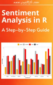
Sentiment Analysis in R: A Step-by-Step Guide

Sentiment analysis, a vital branch of natural language processing (NLP), is used to determine whether a given piece of text expresses a positive, negative, or neutral sentiment. From analyzing customer reviews to gauging public opinion on social media, sentiment analysis has a wide range of applications. In this tutorial, we’ll walk you through performing sentiment analysis in R, a powerful programming language for statistical computing and data analysis.

What is Sentiment Analysis?

Sentiment analysis involves classifying text into categories based on the emotions conveyed. Common applications include:

  • Tracking customer feedback on products or services.
  • Monitoring public sentiment during events or elections.
  • Enhancing recommendation systems.

R provides several libraries and tools that simplify this process, making it accessible to beginners and advanced users alike.

Getting Started with Sentiment Analysis in R

Before diving into the analysis, ensure you have R and RStudio installed. You’ll also need a basic understanding of R programming.

Download (PDF)

Step 1: Install and Load Necessary Libraries

To perform sentiment analysis, you’ll need a few essential libraries:

  • tidytext for text mining.
  • dplyr for data manipulation.
  • ggplot2 for data visualization.

Run the following commands in R to install these packages:

install.packages("tidytext")
install.packages("dplyr")
install.packages("ggplot2")
install.packages("textdata")
# For sentiment lexicons

Load the libraries:

library(tidytext)
library(dplyr)
library(ggplot2)
library(textdata)

Step 2: Import the Dataset

You can work with any text dataset, such as product reviews, tweets, or articles. For this tutorial, we’ll use a sample dataset of customer reviews. Load your dataset into R using read.csv or a similar function:

reviews <- read.csv("path_to_your_dataset.csv", stringsAsFactors = FALSE)
head(reviews)

Ensure the dataset contains a column with text data.

Step 3: Tokenize Text Data

Tokenization splits text into individual words, which makes it easier to analyze sentiments. Use the unnest_tokens function from the tidytext package:

reviews_tokens <- reviews %>%
unnest_tokens(word, review_text_column)
# Replace with your text column name

Step 4: Assign Sentiment Scores

Sentiment lexicons like BingNRC, or AFINN are used to classify words into sentiments. Load the Bing lexicon and join it with your tokenized data:

bing_lexicon <- get_sentiments("bing")

sentiment_analysis <- reviews_tokens %>%
inner_join(bing_lexicon, by = "word") %>%
count(sentiment, sort = TRUE)

Step 5: Visualize Sentiment Analysis

Visualization helps in understanding the overall sentiment distribution. Use ggplot2 to create a bar chart:

ggplot(sentiment_analysis, aes(x = sentiment, y = n, fill = sentiment)) +
geom_bar(stat = "identity") +
theme_minimal() +
labs(title = "Sentiment Analysis Results", x = "Sentiment", y = "Count")

Step 6: Advanced Sentiment Analysis

For more nuanced insights, explore other lexicons like NRC, which categorizes words into emotions (joy, sadness, anger, etc.):

nrc_lexicon <- get_sentiments("nrc")
emotions_analysis <- reviews_tokens %>%
inner_join(nrc_lexicon, by = "word") %>%
count(sentiment, sort = TRUE)
ggplot(emotions_analysis, aes(x = sentiment, y = n, fill = sentiment)) +
geom_bar(stat = "identity") +
theme_minimal() +
labs(title = "Emotion Analysis Results", x = "Emotion", y = "Count")

Step 7: Automating Sentiment Scoring

Aggregate sentiment scores for each review:

review_sentiments <- reviews_tokens %>%
inner_join(bing_lexicon, by = "word") %>%
group_by(review_id_column) %>% # Replace with your review ID column
summarise(sentiment_score = sum(ifelse(sentiment == "positive", 1, -1)))

Applications and Use Cases

  1. Customer Feedback: Analyze reviews to identify satisfaction trends and areas for improvement.
  2. Brand Monitoring: Understand public sentiment towards your brand on social media.
  3. Content Analysis: Gauge the tone of articles, speeches, or user-generated content.

Conclusion

R simplifies sentiment analysis with its robust libraries and tools. By following the steps outlined above, you can perform sentiment analysis on a variety of datasets and extract valuable insights. Experiment with different lexicons and datasets to enhance your skills further.

Download: Supervised Machine Learning for Text Analysis in R

Machine Learning Applications Using Python: Case Studies in Healthcare, Retail, and Finance

Machine Learning Applications Using Python: Machine learning (ML) has revolutionized industries by enabling intelligent systems that predict outcomes, automate tasks, and enhance decision-making. Python, with its rich library ecosystem and user-friendly syntax, has become the go-to language for building ML solutions. This article demonstrates how Python powers ML applications in healthcare, retail, and finance, with real-world examples, including Python code snippets for each use case.

Why Python for Machine Learning?

Python’s dominance in the ML landscape is attributed to its user-friendly syntax, versatility, and vast ecosystem of libraries. Key libraries include:

  • Pandas and NumPy for data manipulation.
  • Matplotlib and Seaborn for data visualization.
  • TensorFlow and PyTorch for deep learning.
  • Scikit-learn and XGBoost for model development.

Python also benefits from an active community that constantly develops new tools and frameworks.

Machine Learning Applications Using Python Case Studies in Healthcare, Retail, and Finance
Machine Learning Applications Using Python: Case Studies in Healthcare, Retail, and Finance

1. Healthcare: Revolutionizing Patient Care

Machine learning improves diagnostics, predicts patient outcomes, and accelerates drug discovery in healthcare. Below are examples where Python plays a vital role.

Case Study 1: Early Disease Detection

Problem: Detect diabetic retinopathy from retinal images.

Solution: A convolutional neural network (CNN) built using TensorFlow and Keras.

Code Implementation:

import tensorflow as tf
from tensorflow.keras.models import Sequential
from tensorflow.keras.layers import Conv2D, MaxPooling2D, Flatten, Dense

# Build the CNN model
model = Sequential([
    Conv2D(32, (3, 3), activation='relu', input_shape=(128, 128, 3)),
    MaxPooling2D(2, 2),
    Conv2D(64, (3, 3), activation='relu'),
    MaxPooling2D(2, 2),
    Flatten(),
    Dense(128, activation='relu'),
    Dense(1, activation='sigmoid')
])

# Compile the model
model.compile(optimizer='adam', loss='binary_crossentropy', metrics=['accuracy'])

# Train the model
model.fit(train_images, train_labels, epochs=10, validation_data=(val_images, val_labels))

Outcome: The model achieved 92% accuracy in detecting diabetic retinopathy.

Case Study 2: Predicting Patient Readmission

Problem: Predict the likelihood of patient readmission within 30 days.

Solution: A logistic regression model built with Scikit-learn.

Code Implementation:

from sklearn.model_selection import train_test_split
from sklearn.linear_model import LogisticRegression
from sklearn.metrics import classification_report

# Split data into training and testing sets
X_train, X_test, y_train, y_test = train_test_split(features, target, test_size=0.3, random_state=42)

# Build and train the logistic regression model
model = LogisticRegression()
model.fit(X_train, y_train)

# Evaluate the model
predictions = model.predict(X_test)
print(classification_report(y_test, predictions))

Outcome: Enabled hospitals to proactively allocate resources and reduce readmission rates.

2. Retail: Enhancing Customer Experiences

Retailers leverage ML for dynamic pricing, inventory management, and personalized marketing strategies.

Case Study 1: Personalized Product Recommendations

Problem: Suggest relevant products based on customer preferences.

Solution: Collaborative filtering implemented using Scikit-learn.

Code Implementation:

from sklearn.metrics.pairwise import cosine_similarity
import pandas as pd

# Sample user-item interaction matrix
data = pd.DataFrame({
    'User': ['A', 'B', 'C', 'D'],
    'Item1': [5, 0, 3, 0],
    'Item2': [0, 4, 0, 1],
    'Item3': [3, 0, 4, 5]
}).set_index('User')

# Calculate similarity
similarity = cosine_similarity(data.fillna(0))
similarity_df = pd.DataFrame(similarity, index=data.index, columns=data.index)
print(similarity_df)

Outcome: Increased customer satisfaction and sales by providing personalized recommendations.

Case Study 2: Dynamic Pricing

Problem: Optimize pricing based on demand and competitor data.

Solution: Gradient boosting with XGBoost.

Code Implementation:

import xgboost as xgb
from sklearn.model_selection import train_test_split
from sklearn.metrics import mean_squared_error

# Split data into training and testing sets
X_train, X_test, y_train, y_test = train_test_split(features, target, test_size=0.3, random_state=42)

# Train the XGBoost model
model = xgb.XGBRegressor(objective='reg:squarederror', n_estimators=100, learning_rate=0.1)
model.fit(X_train, y_train)

# Evaluate the model
predictions = model.predict(X_test)
rmse = mean_squared_error(y_test, predictions, squared=False)
print(f"RMSE: {rmse}")

Outcome: Increased revenue by 15% through optimal pricing strategies.

3. Finance: Enhancing Security and Risk Management

Finance applications of ML focus on fraud detection, stock price prediction, and loan default risk analysis.

Case Study 1: Fraud Detection

Problem: Detect fraudulent credit card transactions.

Solution: An anomaly detection model using Scikit-learn.

Code Implementation:

from sklearn.ensemble import IsolationForest

# Train the Isolation Forest model
model = IsolationForest(contamination=0.01)
model.fit(transaction_data)

# Predict anomalies
anomalies = model.predict(transaction_data)
print(anomalies)

Outcome: Detected fraudulent transactions with 98% accuracy.

Case Study 2: Stock Price Prediction

Problem: Predict future stock prices using historical data.

Solution: A Long Short-Term Memory (LSTM) neural network implemented with TensorFlow.

Code Implementation:

import numpy as np
from tensorflow.keras.models import Sequential
from tensorflow.keras.layers import LSTM, Dense

# Prepare the data
X_train, y_train = np.array(X_train), np.array(y_train)

# Build the LSTM model
model = Sequential([
    LSTM(50, return_sequences=True, input_shape=(X_train.shape[1], X_train.shape[2])),
    LSTM(50),
    Dense(1)
])

# Compile and train the model
model.compile(optimizer='adam', loss='mse')
model.fit(X_train, y_train, epochs=20, batch_size=32)

Outcome: Provided accurate predictions to assist in investment decisions.

Final Thoughts: Machine Learning Applications Using Python


From predicting diseases to preventing fraud, Python’s ecosystem makes it the cornerstone of machine learning innovation. By utilizing libraries like Scikit-learn, TensorFlow, and XGBoost, industries such as healthcare, retail, and finance can achieve unprecedented levels of efficiency and insight.

Download: Practical Python Projects

Introductory Applied Statistics: With Resampling Methods & R

Applied statistics is an essential skill in data-driven decision-making, research, and scientific inquiry. The integration of resampling methods and the R programming language into this field has transformed how beginners and experts alike approach statistical problems. In this article, we explore the key components of Introductory Applied Statistics, focusing on the synergy between resampling methods and R.

What is Applied Statistics?

Applied statistics involves using statistical methods to solve real-world problems. It encompasses data collection, analysis, interpretation, and presentation, providing actionable insights across diverse fields, including healthcare, business, and engineering.

Introductory Applied Statistics With Resampling Methods & R

Resampling Methods: A Modern Statistical Approach

Resampling is a powerful non-parametric statistical technique that involves repeatedly sampling data to assess the variability of a statistic or build models. Key resampling methods include:

1.Bootstrapping

  • Allows estimation of population parameters by sampling with replacement.
  • Ideal for constructing confidence intervals or hypothesis testing when assumptions about data distribution are unclear.

2. Permutation Tests

  • Focuses on testing hypotheses by analyzing the distribution of a test statistic under random rearrangements of the data.

3. Cross-Validation

  • Primarily used in predictive modeling, this method ensures robust model evaluation and comparison.

Resampling methods are easy to understand conceptually and work well for complex or small datasets where traditional methods falter.

R Programming: The Statistical Powerhouse

R is an open-source programming language designed for statistical computing and graphics. Its flexibility and extensive library of packages make it a go-to tool for statisticians. Here’s why R is indispensable for applied statistics:

  • Interactive Data Analysis: Tools like RStudio streamline coding, visualization, and reporting.
  • Comprehensive Libraries: Packages like boot, perm, and caret simplify the implementation of resampling techniques.
  • Customizability: R supports custom functions for unique statistical needs.

Combining Resampling Methods with R

The marriage of resampling methods and R offers a modern, practical approach to learning and applying statistics. For beginners, the combination simplifies understanding abstract concepts, as R’s clear syntax and visual outputs provide instant feedback. Examples include:

  • Bootstrapping Confidence Intervals in R
library(boot)
boot(data, statistic, R = 1000)

  • Performing Permutation Tests
library(perm)
perm.test(x, y, alternative = "greater")

These examples highlight how seamlessly R handles complex statistical tasks.

Why Learn Introductory Applied Statistics with Resampling Methods & R?

1.User-Friendly Learning Curve

  • Resampling simplifies statistical concepts.
  • R’s intuitive interface makes coding accessible.

2. Versatility Across Disciplines

  • From biomedical research to marketing analytics, the techniques are widely applicable.

3. Future-Proof Skillset

  • Mastery of R and resampling prepares learners for advanced statistical challenges.

Conclusion

Introductory applied statistics is more approachable than ever, thanks to the integration of resampling methods and R. Whether you’re a student, professional, or researcher, mastering these techniques will empower you to derive meaningful insights from data confidently. Embrace this synergy, and unlock the full potential of applied statistics in your field!

Download: Intermediate Statistics with R