Data Science Archives - Page 37 of 45

Learn R for Applied Statistics: With Data Visualizations, Regressions, and Statistics

Learn R for Applied Statistics: With Data Visualizations, Regressions, and Statistics: Learning R for applied statistics can be a great way to gain insights into data analysis and modeling. It provides a wide range of statistical techniques, including linear and nonlinear modeling, time-series analysis, and multivariate analysis. R is also popular among researchers for data visualization and exploratory data analysis. With its open-source nature and active community, R offers extensive documentation and various packages, making it a powerful tool for statistical analysis and modeling in fields such as economics, biology, social sciences, and more. Its flexibility and ease of use make it an excellent choice for researchers and data analysts of all levels.

R provides several libraries and packages for regression analysis, making it an excellent tool for applied statistics. With its active community and extensive documentation, R is an excellent choice for researchers, data analysts, and scientists of all levels. One of the most widely used libraries for regression analysis in R is the “lm” function. It is used for linear regression and helps users to fit a linear model to a given set of data. The package provides users with several diagnostic measures such as the R-squared value, residual plots, and coefficients. Another popular library for regression analysis in R is the “glm” function.

The package helps users to fit generalized linear models to a given set of data. The package provides a wide range of regression models such as logistic regression, Poisson regression, and negative binomial regression. The “car” library is another popular package for regression analysis in R. It provides several diagnostic tools and regression models such as ANOVA, MANOVA, and multiple regression. Finally, the “caret” package provides various machine learning algorithms, including regression analysis. The package helps users to train, test, and evaluate regression models and provides several techniques to handle missing data and outliers.

R is an excellent tool for data visualization and exploratory data analysis, offering various packages and libraries for creating high-quality graphics. With its powerful graphics capabilities and active community, R is an excellent choice for researchers, data analysts, and scientists of all levels. R’s ggplot2 package is one of the most widely used libraries for creating data visualizations. It provides a flexible and elegant system for creating complex and informative graphics. Its grammar of graphics approach allows users to create a wide range of visualizations using a consistent set of rules.

Other popular R packages for data visualization include plotly, lattice, and ggvis. Plotly provides interactive visualizations that allow users to explore data in real time, while lattice offers a powerful and flexible system for creating multi-panel plots. ggvis, on the other hand, provides an interactive grammar of graphics system for creating complex visualizations with interactivity.

Download(PDF)

March 30, 2023 by SAROJ Books Data Science

How to make a boxplot in R?

A box plot is a graphical representation of a dataset that displays the distribution of data through five summary statistics: the minimum value, the first quartile (25th percentile), the median (50th percentile), the third quartile (75th percentile), and the maximum value. The box in the plot represents the middle 50% of the data (between the first and third quartiles), while the whiskers extend from the box to show the range of the data, excluding any outliers. Outliers are represented by dots or asterisks outside the whiskers. Box plots are useful for quickly visualizing the spread, skewness, and outliers of a dataset. They are commonly used in statistical analysis, especially for comparing distributions between different groups or variables.

To make a boxplot in R, you can use the boxplot() function, which is a built-in function in R. Here’s an example code:

# Create a vector of data
data <- c(10, 20, 15, 30, 25, 35, 40, 50)

# Create a boxplot of the data
boxplot(data)

In the above example, we first create a vector of data called data. Then we use the boxplot() function to create a boxplot of the data.

You can customize the boxplot by adding different parameters to the boxplot() function. Here are some examples:

Adding a title to the plot:

boxplot(data, main="Boxplot of Data")

Changing the x-axis label:

boxplot(data, xlab="Data")

Changing the color of the box and whiskers:

boxplot(data, col="blue")

Creating a horizontal boxplot:

boxplot(data, horizontal=TRUE)

These are just a few examples of how you can customize the boxplot in R. You can find more information about the boxplot() function and its parameters in the R documentation.

Download (PDF)

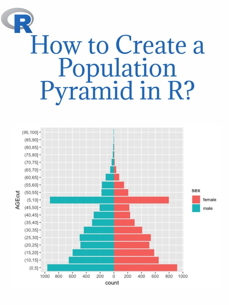
March 30, 2023 by SAROJ Data Science

How to Create a Population Pyramid in R?

An age-sex pyramid is also known as a population pyramid. Using it, we can visualize the distribution of a population by age group and gender. In general, it resembles a pyramid. Females are represented on the right of the population pyramid, while males are typically depicted on the left. Based on the number or percentage of men and women in a particular population, this data visualization method can be used to visualize that population’s age. Creating a population pyramid in R is a common data analysis and visualization task. Here are the steps to create a population pyramid in R:

Download:

Step 1: Install and load necessary packages Before starting to create a population pyramid, we need to install and load the ggplot2 and dplyr packages. These packages are used for data visualization and data manipulation, respectively.

install.packages("ggplot2")
install.packages("dplyr")

library(ggplot2)
library(dplyr)

Step 2: Load the Data To create a population pyramid, we need data on the age and sex distribution of the population. We can use the built-in “midwest” dataset from ggplot2 package as an example.

data(midwest)

Step 3: Data Wrangling Next, we need to prepare the data for the population pyramid visualization. We will use the dplyr package to manipulate the data.

midwest <- midwest %>%
  select(county, state, Poptotal, popdensity, percwhite, percblack, percamericanindian, percasian, perchispanic, percother, medianage, medianhousevalue, medianincome, region, division) %>%
  filter(!is.na(Poptotal), !is.na(medianage)) %>%
  mutate_at(vars(percwhite:percother), ~replace_na(., 0))

Step 4: Create the Population Pyramid Now, we can create the population pyramid using the ggplot2 package.

ggplot(midwest, aes(x = medianage, y = Poptotal, fill = factor(ifelse(medianage < 37.5, "Male", "Female")))) +
  geom_bar(stat = "identity", position = "identity") +
  scale_fill_manual(values = c("#619CFF", "#FF6161")) +
  labs(title = "Population Pyramid", x = "Median Age", y = "Population", fill = "") +
  coord_flip()

This will create a population pyramid in R, showing the age and sex distribution of the population.

The above example is just a sample, and you can use your own data to create the population pyramid in R.

Download (PDF)

March 29, 2023 by SAROJ Data Science

Create A Dashboard In R

There are several ways to create a dashboard in R, but one of the most popular and powerful options is to use the Shiny package. Shiny allows you to build interactive web applications directly from R code, including data visualization and analysis. Here are the general steps to creating a dashboard in R using Shiny:

Install and load the Shiny package:

install.packages("shiny")
library(shiny)

Load your data: You can use any data source that you like, but it’s important to make sure that the data is in a format that can be used by Shiny.
Create a user interface (UI): This is where you define what the user will see and interact with in your dashboard. You can use Shiny’s built-in UI elements (such as sliders, drop-down menus, and text boxes) or create your own custom UI elements using HTML, CSS, and JavaScript.
Create a server function: This is where you define the logic and calculations that will power your dashboard. You can use any R code you like, including data manipulation and analysis functions.
Combine the UI and server: Use the shinyApp() function to combine the UI and server functions into a complete Shiny application.
Deploy your dashboard: You can deploy your Shiny dashboard to a variety of platforms, including shinyapps.io and your own web server.

Here’s a basic example of a Shiny dashboard that displays a histogram of a dataset:

# Load the Shiny package
library(shiny)

# Load the dataset
data(mtcars)

# Define the UI
ui <- fluidPage(
  titlePanel("MTCars Histogram"),
  sidebarLayout(
    sidebarPanel(
      sliderInput("bins", "Number of bins:", min = 1, max = 50, value = 30)
    ),
    mainPanel(
      plotOutput("histogram")
    )
  )
)

# Define the server
server <- function(input, output) {
  output$histogram <- renderPlot({
    bins <- seq(min(mtcars$mpg), max(mtcars$mpg), length.out = input$bins + 1)
    hist(mtcars$mpg, breaks = bins, col = "blue", main = "MTCars Histogram")
  })
}

# Combine the UI and server
shinyApp(ui = ui, server = server)

This code creates a Shiny app with a slider that allows the user to control the number of bins in a histogram of the mpg column of the mtcars dataset. When the user moves the slider, the histogram is updated in real-time. You can customize this example and add more elements to create a full dashboard with multiple charts, tables, and other interactive features.

Download:

March 27, 2023 by SAROJ Data Science

Geographic Data Science with R

Geographic Data Science with R is a powerful tool for analyzing and visualizing spatial data. It allows you to combine statistical analysis with geographic information, allowing you to better understand the patterns and relationships in your data. One of the key benefits of Geographic Data Science with R is its ability to handle large and complex data sets. With R’s powerful tools for data manipulation and visualization, you can quickly explore and analyze large data sets without sacrificing accuracy or speed. Another advantage of Geographic Data Science with R is the ability to work with a wide range of data formats, including raster and vector data. This flexibility makes it easier to work with data from a variety of sources and to integrate different types of data into your analysis. Visualizing and analyzing environmental change is an important application of Geographic Data Science with R. Here are some steps you can follow to get started:

Read Now

Acquire data: Start by collecting environmental data relevant to your study, such as temperature, precipitation, land cover, or vegetation indices. Many sources provide this type of data for free or for a fee, such as NASA, NOAA, or USGS.

Pre-process the data: Once you have obtained the data, you may need to pre-process it to prepare it for analysis. This may include converting data formats, aggregating or disaggregating data to match the scale of your analysis, or removing missing values.

Visualize the data: Use R’s powerful visualization tools to create maps, charts, and other visualizations of the data. For example, you can create heat maps to visualize temperature patterns or time series plots to track changes over time. Interactive maps can also be created using tools such as Leaflet or Shiny.

Analyze the data: Use statistical tools in R to analyze the data and identify patterns or trends. For example, you can use regression analysis to identify relationships between environmental variables, or cluster analysis to identify groups of locations with similar environmental conditions.

Interpret and communicate the results: Once you have analyzed the data, interpret the results and communicate them effectively to stakeholders, policymakers, or the public. Use visualizations and summaries to effectively communicate your findings.

Download:

March 25, 2023 by SAROJ Books Data Science

Confidence Intervals in R

A confidence interval is a range of values that provides a plausible range of values for an unknown population parameter, based on a sample from that population. The confidence interval is expressed as a percentage, such as 95% or 99%, which represents the level of confidence you have that the true population parameter falls within the interval. For example, if you calculate a 95% confidence interval for the average height of students in the school, you can say with 95% confidence that the true average height falls within that range of values. Calculating confidence intervals using R is relatively simple. Here’s a general process you can follow:

Download:

Load your data into R. You can do this by typing the name of your data file, followed by the read.table() function, like this: mydata <- read.table("myfile.txt", header=TRUE). This assumes that your data is in a tab-delimited text file with headers.
Calculate the sample mean and standard deviation. You can use the mean() and sd() functions in R to do this, like this: mymean <- mean(mydata$myvariable) and mysd <- sd(mydata$myvariable). Replace “myvariable” with the name of the variable in your data that you want to calculate the confidence interval for.
Determine the sample size. You can use the nrow() function in R to get the number of rows (i.e., observations) in your data, like this: mysize <- nrow(mydata).
Choose a confidence level. You’ll need to decide on a confidence level for your confidence interval. For example, you might choose 95%, which is a common level of confidence.
Calculate the confidence interval. You can use the t.test() function in R to calculate the confidence interval, like this: myci <- t.test(mydata$myvariable, conf.level=0.95)$conf.int. This will give you a 95% confidence interval for the mean of your variable.
Print or save the confidence interval. You can use the print() function to print the confidence interval to the console, like this: print(myci). Or you can save it to a variable and use it later in your code, like this: myci <- t.test(mydata$myvariable, conf.level=0.95)$conf.int.

Keep in mind that the exact method of calculating the confidence interval may vary depending on the type of data you’re working with and the statistical test you’re using. But the general process outlined above should give you a good starting point for calculating confidence intervals in R.

Data Analysis and Visualization Using Python

Python is a popular programming language for data analysis and visualization due to its versatility and a large number of libraries specifically designed for these tasks. Here are the basic steps to perform data analysis and visualization using Python:

Download:

Import the required libraries: The most commonly used libraries for data analysis and visualization in Python are Pandas, Matplotlib, and Seaborn. You can import them using the following code:

import pandas as pd
import matplotlib.pyplot as plt
import seaborn as sns

Load the data: Once the libraries are imported, you can load the data into a Pandas DataFrame. Pandas provides several functions to read data from different sources, such as CSV files, Excel files, SQL databases, etc. For example, to read a CSV file named ‘data.csv’, you can use the following code:

data = pd.read_csv('data.csv')

Explore the data: Before visualizing the data, it is important to explore it to understand its structure and characteristics. You can use Pandas functions like head(), tail(), describe(), info(), etc. to get a summary of the data.

print(data.head())
print(data.describe())
print(data.info())

Clean the data: If the data contains missing or inconsistent values, you need to clean it before visualizing it. Pandas provides functions to handle missing values and outliers, such as dropna(), fillna(), replace(), etc.

data.dropna(inplace=True) # remove rows with missing values
data.replace({'gender': {'M': 'Male', 'F': 'Female'}}, inplace=True) # replace inconsistent values

Visualize the data: Once the data is cleaned and prepared, you can start visualizing it using Matplotlib and Seaborn. Matplotlib provides basic visualization functions like plot(), scatter(), hist(), etc., while Seaborn provides more advanced functions for statistical data visualization, such as distplot(), boxplot(), heatmap(), etc. Here’s an example of creating a histogram of age distribution using Seaborn:

sns.distplot(data['age'], bins=10)
plt.title('Age Distribution')
plt.xlabel('Age')
plt.ylabel('Density')
plt.show()

These are the basic steps of course, there are many more advanced techniques and libraries available, depending on your specific needs and goals.

Download(PDF)

March 23, 2023 by SAROJ Books Data Science

Line graph with R

A line graph is a type of chart used to display data as a series of points connected by lines. It is commonly used to show trends over time or to compare multiple data sets. Line graphs are useful for visualizing data that changes continuously over time, such as stock prices, weather patterns, or population growth. They can also be used to compare multiple data sets, such as the performance of different companies in a particular industry. To create a line graph in R, you can use the built-in plot() function or the more powerful ggplot2 library. Here is an example of how to create a line graph using ggplot2.

First, let’s create a sample data frame with some random values:

# Create sample data frame
x <- 1:10
y <- c(3, 5, 6, 8, 10, 12, 11, 9, 7, 4)
df <- data.frame(x, y)

Next, we’ll use ggplot() to create a plot object, and then add a geom_line() layer to draw the line:

# Load ggplot2 library
library(ggplot2)

# Create plot object
p <- ggplot(df, aes(x, y))

# Add line layer
p + geom_line()

This will create a basic line graph with the x values on the x-axis and the y values on the y-axis. You can customize the appearance of the graph by adding additional layers or modifying the ggplot() object. For example, you can add axis labels and a title:

# Add axis labels and title
p + geom_line() + 
  labs(x = "X-axis label", y = "Y-axis label", title = "Title of the graph")

You can also modify the line color and thickness using the color and size arguments of geom_line():

# Change line color and thickness
p + geom_line(color = "red", size = 2) +
  labs(x = "X-axis label", y = "Y-axis label", title = "Title of the graph")

These are just a few examples of the many customization options available in ggplot2.

Download(PDF)

March 22, 2023 by SAROJ Data Science

Data Structures and Algorithms with Python

Data structures and algorithms are fundamental concepts in computer science and software engineering. They help us solve problems more efficiently by organizing and manipulating data in a way that allows for faster retrieval and processing. Python is a popular programming language that is widely used for data analysis, scientific computing, web development, and many other applications. It provides a rich set of built-in data structures and libraries that make it easy to implement common algorithms and data structures.

Download:

Some of the commonly used data structures in Python include lists, tuples, sets, and dictionaries. Lists are mutable sequences of elements, tuples are immutable sequences, sets are unordered collections of unique elements, and dictionaries are mappings between keys and values.

There are also several libraries in Python that provide more advanced data structures and algorithms, such as NumPy, Pandas, and Scikit-learn for data analysis and machine learning, and NetworkX for graph algorithms.

When it comes to algorithms, Python provides a rich set of built-in functions and libraries that make it easy to implement common algorithms, such as sorting, searching, and graph traversal. Some of the popular algorithms that are commonly implemented in Python include binary search, quicksort, mergesort, and breadth-first search.

To master data structures and algorithms with Python, it is important to have a good understanding of the fundamental concepts, as well as the specific features and libraries provided by the language. It is also helpful to practice implementing algorithms and data structures in Python and to study examples and tutorials from experienced programmers and online resources.

Download(PDF)

March 21, 2023 by SAROJ Books Data Science

Statistics and Data Analysis for Financial Engineering

Statistics and data analysis are essential skills for financial engineering, as they provide the foundation for modeling and analyzing financial data. R is a popular programming language for data analysis and statistical modeling, and it has numerous packages that are well-suited for financial engineering applications. Here are some key areas where statistics and data analysis can be applied in financial engineering using R:

Download:

Risk Analysis: Financial engineers use statistical methods to estimate the likelihood of different types of risks, such as market risk, credit risk, and operational risk. R has several packages like “Risk” and “fBasics” that can be used to perform different types of risk analysis.

Time Series Analysis: Financial time series data typically exhibit patterns such as trends, seasonality, and autocorrelation. R has several packages like “tseries” and “forecast” that are specifically designed for analyzing time series data.

Portfolio Optimization: Financial engineers use statistical methods to optimize investment portfolios by balancing risk and return. R has several packages like “PortfolioAnalytics” and “quantmod” that can be used to perform portfolio optimization.

Monte Carlo Simulation: Monte Carlo simulation is a powerful statistical technique used to model complex systems and estimate probabilities. In finance, Monte Carlo simulation is used to estimate the value of financial derivatives and to simulate the behavior of financial markets. R has several packages like “mc2d” and “MCMCpack” that can be used for Monte Carlo simulation.

Data Visualization: Data visualization is an important part of data analysis in financial engineering. R has several packages like “ggplot2” and “lattice” that can be used to create visualizations of financial data.

Download(PDF)

March 21, 2023 by SAROJ Books Data Science

Data Science

Recent Posts

Books