PYOFLIFE

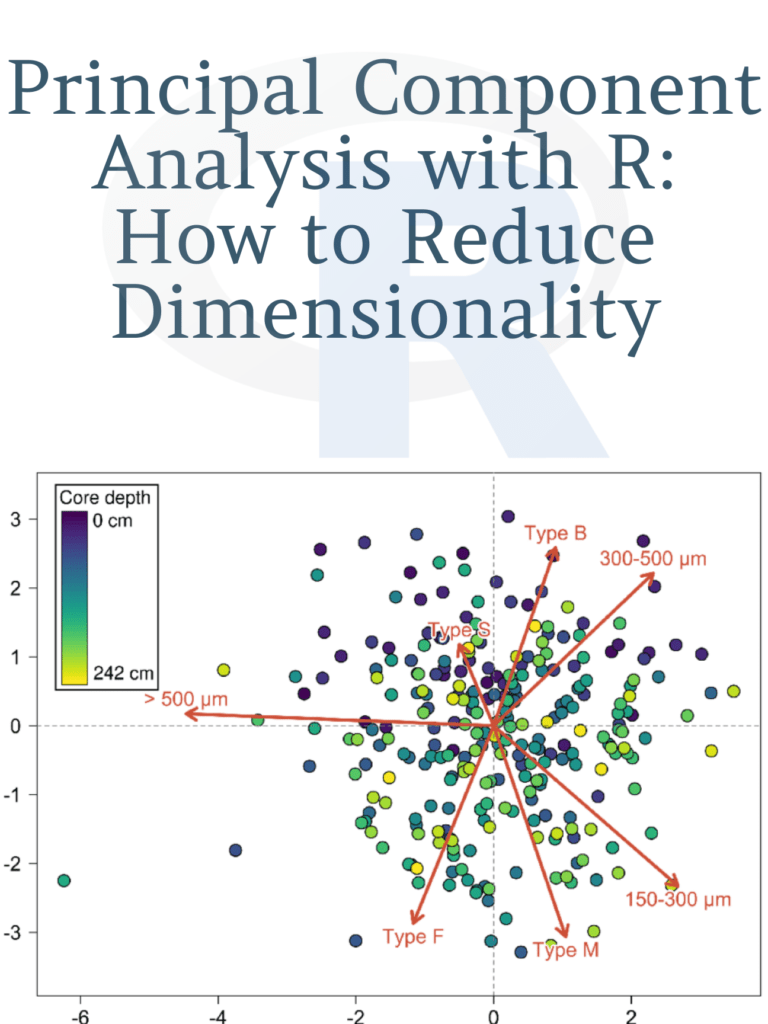
Understanding R Object Types: If you’re new to R, one of the first things you’ll need to understand is the concept of object types. R is a dynamically-typed language, meaning that objects are not assigned a specific type at the time of declaration, but rather their type is determined at runtime. In this article, we’ll cover the different types of objects in R, how to create and manipulate them, and how to work with their associated functions.

Table of Contents

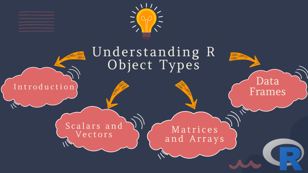
1. Introduction
2. Scalars and Vectors
   • Numeric Vectors
   • Integer Vectors
   • Complex Vectors
   • Logical Vectors
   • Character Vectors
   • Factor Vectors
3. Matrices and Arrays
4. Lists
5. Data Frames
6. FAQs

1. Introduction

R is a powerful programming language used extensively for data analysis and statistical computing. One of its key features is its ability to work with a variety of object types. In R, objects can be anything from a single number to a complex data structure containing many elements.

2. Scalars and Vectors

Scalars are single values in R, such as a number or character string. Vectors are collections of scalars of the same type, arranged in a specific order.

Numeric Vectors

Numeric vectors are the most common type of vector in R, and can contain any real number. They are created using the c() function:

> x <- c(1.5, 2.7, 3.9)
> x
[1] 1.5 2.7 3.9

Integer Vectors

Integer vectors can contain only whole numbers. They are created using the as.integer() function:

> y <- as.integer(c(1, 2, 3))
> y
[1] 1 2 3

Complex Vectors

Complex vectors are used to represent complex numbers, which have both real and imaginary component. They are created using the c() function with the complex() function:

> z <- c(1+2i, 2+3i, 3+4i)
> z
[1] 1+2i 2+3i 3+4i

Logical Vectors

Logical vectors contain either TRUE or FALSE values, and are used extensively in conditional statements. They are created using the c() function:

> a <- c(TRUE, FALSE, TRUE)
> a
[1]  TRUE FALSE  TRUE

Character Vectors

Character vectors contain text strings. They are created using the c() function with quotes:

> b <- c("apple", "banana", "cherry")
> b
[1] "apple"  "banana" "cherry"

Factor Vectors

Factor vectors are used to represent categorical data. They are created using the factor() function:

> c <- factor(c("red", "green", "blue"))
> c
[1] red   green blue 
Levels: blue green red

3. Matrices and Arrays

Matrices are two-dimensional collections of data, while arrays can have any number of dimensions. They are created using the matrix() and array() functions:

> m <- matrix(c(1, 2, 3, 4, 5, 6), nrow=2, ncol=3)
> m
     [,1] [,2] [,3]
[1,]    1    3    5
[2,]    2    4    6

Arrays are similar to matrices but can have more than two dimensions. Here is an example of a three-dimensional array:

> a <- array(c(1, 2, 3, 4, 5, 6, 7, 8), dim=c(2, 2, 2))
> a
, , 1

     [,1] [,2]
[1,]    1    3
[2,]    2    4

, , 2

     [,1] [,2]
[1,]    5    7
[2,]    6    8

4. Lists

Lists are one of the most versatile object types in R. They can contain objects of different types and sizes, and can even contain other lists. They are created using the list() function:

> l <- list(1, "apple", c(1, 2, 3))
> l
[[1]]
[1] 1

[[2]]
[1] "apple"

[[3]]
[1] 1 2 3

5. Data Frames

Data frames are used to represent tabular data, such as spreadsheets or database tables. They are similar to matrices but can contain columns of different types. They are created using the data.frame() function:

> df <- data.frame(name=c("Alice", "Bob", "Charlie"), age=c(25, 30, 35), married=c(TRUE, FALSE, TRUE))
> df
     name age married
1   Alice  25    TRUE
2     Bob  30   FALSE
3 Charlie  35    TRUE

6. FAQs

1. What is the difference between a scalar and a vector in R?
   • A scalar is a single value, while a vector is a collection of values of the same type.
2. How do I create a matrix in R?
   • You can create a matrix using the matrix() function.
3. What is a data frame in R?
   • A data frame is a type of object used to represent tabular data, such as spreadsheets or database tables.
4. What is a factor in R?
   • A factor is a type of vector used to represent categorical data.
5. Why is it important to choose the right type of object in R?
   • The type of an object can affect how it is treated by R functions, so choosing the right type is important to ensure correct results.

Download: Beginning Data Science in R: Data Analysis, Visualization, and Modelling for the Data Scientist

Creating Violin Plots Using R: Violin plots are a popular method for visualizing the distribution of a dataset. These plots are similar to box plots but provide a more detailed view of the distribution by showing the density of the data at different values. In this article, we will discuss how to create violin plots using R and how to interpret them.

To begin, we will need a dataset to work with. For this example, we will use the “mtcars” dataset which is built into R. This dataset contains information on various attributes of 32 cars, including their miles per gallon (mpg), number of cylinders (cyl), and horsepower (hp). We will focus on the mpg variable for our example.

First, let’s load the dataset into R:

data(mtcars)

Now, let’s create a simple violin plot of the mpg variable:

library(ggplot2)
ggplot(mtcars, aes(x = "", y = mpg)) + 
  geom_violin()

This will produce a basic violin plot of the mpg variable. The x-axis is left blank because we are not grouping the data by any variable. The y-axis shows the values of the mpg variable, and the width of the violin at each point indicates the density of the data at that value. The thicker portions of the violin indicate where the data is more densely distributed.

We can customize the plot in several ways. For example, we can color the violins based on the number of cylinders in each car:

ggplot(mtcars, aes(x = factor(cyl), y = mpg, fill = factor(cyl))) + 
  geom_violin()

This will produce a violin plot with each violin colored based on the number of cylinders in each car. We can see that cars with 4 cylinders tend to have higher mpg values than cars with 6 or 8 cylinders.

We can also overlay a box plot on the violin plot to show additional information about the distribution:

ggplot(mtcars, aes(x = factor(cyl), y = mpg, fill = factor(cyl))) + 
  geom_violin() +
  geom_boxplot(width = 0.1, fill = "white")

This will produce a violin plot with a box plot overlaid on top of it. The box plot shows the median, quartiles, and any outliers in the data.

Learn: How to create a heat map on R programming?

Hypothesis testing is a statistical technique used to make decisions about a population based on a sample of data. It is a crucial part of data analysis and can be used to test whether a particular hypothesis or assumption is true or not. R is a popular programming language used for data analysis and is equipped with numerous tools and functions to perform hypothesis testing. In this article, we will discuss the steps involved in performing hypothesis testing with R.

Step 1: Define the Hypothesis

The first step in hypothesis testing is to define the null hypothesis and the alternative hypothesis. The null hypothesis is the statement that we are testing, and the alternative hypothesis is the opposite of the null hypothesis. For example, let’s say we want to test whether the average height of students in a class is 5 feet. Our null hypothesis would be that the average height of students is equal to 5 feet, and the alternative hypothesis would be that the average height of students is not equal to 5 feet.

Step 2: Collect Data

The next step is to collect data. This involves selecting a sample from the population and recording the necessary data. In our example, we would measure the height of a random sample of students in the class.

Step 3: Choose a Statistical Test

The third step is to choose an appropriate statistical test to perform hypothesis testing. The choice of test depends on the type of data and the nature of the hypothesis being tested. In R, there are several built-in functions for performing various statistical tests such as t-tests, ANOVA, chi-squared tests, etc. For our example, we will use the t-test since we are testing the difference between the means of the two groups.

Step 4: Conduct the Test

After selecting the appropriate test, we can conduct the test using the corresponding R function. For example, to conduct a two-sample t-test in R, we can use the t.test() function. We can pass the data as arguments to the function along with the null and alternative hypotheses.

Here is an example of how to conduct a two-sample t-test in R:

# Generate sample data
group1 <- rnorm(20, 68, 2) # group 1 with mean 68 and sd 2
group2 <- rnorm(20, 72, 2) # group 2 with mean 72 and sd 2

# Perform two-sample t-test
t.test(group1, group2, alternative = "two.sided", mu = 0, paired = FALSE)

In this example, we generated two random samples of size 20 with means 68 and 72, respectively. We then used the t.test() function to perform a two-sample t-test, specifying the alternative hypothesis as two-sided and the null hypothesis as 0. The output of the function will provide us with the test statistic, p-value, and confidence interval.

Step 5: Interpret the Results

The final step is to interpret the results of the hypothesis test. The output of the test will provide us with a p-value, which is the probability of obtaining the observed sample mean difference (or more extreme) if the null hypothesis is true. If the p-value is less than the significance level (usually 0.05), we can reject the null hypothesis and accept the alternative hypothesis. If the p-value is greater than the significance level, we fail to reject the null hypothesis.

In conclusion, hypothesis testing is an essential part of data analysis, and R provides numerous tools and functions to perform hypothesis testing. By following the steps outlined above, we can perform hypothesis testing in R and make informed decisions based on the results of our tests.

Learn: Confidence Intervals in R

Survival analysis is a statistical technique used to analyze time-to-event data, such as the time until death or the time until the failure of a machine. R is a popular programming language used by statisticians and data analysts for data analysis, visualization, and modeling.

In R, survival analysis can be performed using the survival package. This package provides functions for fitting different types of survival models and for conducting various types of survival analyses, such as Kaplan-Meier curves, Cox proportional hazards regression, and parametric survival models.

To begin, you will need to load the survival package into R by typing:

library(survival)

The first step in survival analysis is to create a survival object. A survival object is a data structure that contains information about the time-to-event data, including the time-to-event (often called “survival time”), the event status (often called “censoring status”), and any covariates that may affect the survival time.

To create a survival object, you can use the Surv() function. For example, suppose you have a dataset called mydata that contains information on the survival time and censoring status of patients in a clinical trial. You can create a survival object as follows:

my.survival <- Surv(time = mydata$time, event = mydata$status)

In this example, time is a vector of survival times, and status is a vector of censoring statuses (0 if the event was censored, 1 if the event occurred). The Surv() function combines these vectors into a single survival object.

Once you have created a survival object, you can use it to fit survival models. The most commonly used survival model is the Cox proportional hazards regression model, which allows you to estimate the effect of covariates on the hazard rate (i.e., the instantaneous risk of experiencing the event at any given time). To fit a Cox proportional hazards model in R, you can use the coxph() function. For example:

my.coxph <- coxph(formula = Surv(time, status) ~ covariate1 + covariate2, data = mydata)

In this example, formula is a formula that specifies the survival object and the covariates to be included in the model, and data is the name of the dataset containing the variables. The output of the coxph() function is an object of class “coxph”, which can be used to obtain estimates of the hazard ratio (i.e., the relative hazard of experiencing the event associated with a one-unit increase in a covariate) and other model parameters.

In addition to Cox proportional hazards regression, there are many other types of survival models that can be fitted using the survival package, such as parametric survival models, accelerated failure time models, and frailty models. The package also provides functions for conducting various types of survival analyses, such as Kaplan-Meier curves and log-rank tests.

Overall, survival analysis is a powerful method for analyzing time-to-event data in R, and the survival package provides a wide range of functions and tools for conducting different types of survival analyses.

Learn: Principal Component Analysis with R: How to Reduce Dimensionality

As a student of data analysis, we understand that Principal Component Analysis (PCA) is a powerful tool that helps reduce the dimensionality of large datasets while retaining the most relevant information. PCA is widely used in various fields such as finance, biology, and image processing. In this article, we will guide you through the process of performing PCA using R, a popular statistical software.

Understanding Principal Component Analysis

PCA is a statistical method used to reduce the number of variables in a dataset while retaining the most important information. It works by transforming the original variables into a new set of uncorrelated variables, called principal components. These principal components are ordered in terms of the amount of variance they explain in the original data.

Performing PCA with R

In this section, we will show you how to perform PCA using R. We will use the iris dataset, which is included in the base R installation. The iris dataset contains measurements of the sepal length, sepal width, petal length, and petal width of three different species of iris flowers.

First, we load the iris dataset into R:

data(iris)

Next, we standardize the variables to have a mean of 0 and a standard deviation of 1, which is necessary for PCA:

irisscale <- scale(iris[,1:4])

Now, we can perform PCA on the standardized iris dataset:

irispca <- prcomp(irisscale)

The prcomp() function in R performs PCA and returns a list of objects. The most important object in the list is the rotation matrix, which contains the principal components.

Visualizing the Results of PCA

To visualize the results of PCA, we can create a scree plot, which shows the amount of variance explained by each principal component. We can create a scree plot using the following code:

plot(irispca)

This will create a plot that shows the proportion of variance explained by each principal component. The x-axis represents the principal components, and the y-axis represents the proportion of variance explained.

Next, we can create a biplot, which shows the relationship between the variables and the principal components. We can create a biplot using the following code:

biplot(irispca)

This will create a plot that shows the variables as arrows and the observations as points. The length and direction of the arrows represent the contribution of each variable to the principal components.

Download: Introduction to Scientific Programming and Simulation using R

Download(PDF)

Cluster Analysis with R: How to Group Similar Data Points: Cluster analysis is a statistical technique used to group similar data points into clusters or segments. It is a useful tool in data analysis, especially when dealing with large datasets, to identify patterns and structure within the data. Cluster analysis can be applied to various fields, such as marketing, biology, and social sciences. In this article, we will explore how to perform cluster analysis using the R programming language.

Types of Clustering

There are two main types of clustering techniques, hierarchical and partitioning. Hierarchical clustering creates a tree-like structure that shows the relationship between data points, whereas partitioning clustering divides data into distinct clusters based on certain criteria. In this article, we will focus on the partitioning clustering technique, specifically k-means clustering.

K-Means Clustering

K-means clustering is a popular partitioning clustering technique used to group data points into K clusters. The K-means algorithm works by minimizing the sum of squared distances between each data point and the centroid of its cluster. The centroid is the center point of each cluster.

To perform k-means clustering in R, we first need to install and load the “stats” package. This package contains the “kmeans” function that we will use to cluster our data.

install.packages("stats")
library(stats)

Next, we need to import our data into R. For this example, we will use the built-in “iris” dataset that contains measurements of three different species of iris flowers.

data(iris)
head(iris)

The “iris” dataset contains four numeric variables: Sepal. Length, Sepal.Width, Petal.Length, and Petal.Width. We will use these variables to cluster the iris flowers into K groups.

To perform k-means clustering on the iris dataset, we need to specify the number of clusters we want to create. In this example, we will create three clusters since there are three species of iris flowers in the dataset.

set.seed(123)
kmeans_result <- kmeans(iris[,1:4], centers = 3)

The “kmeans” function takes two arguments, the first argument is the dataset, and the second argument is the number of clusters we want to create. We also set the seed value to ensure that our results are reproducible.

We can access the results of our clustering analysis by calling the “kmeans_result” object. The “kmeans_result” object contains several components, including the cluster centers and the cluster assignments for each data point.

kmeans_result$centers
kmeans_result$cluster

The “centers” component contains the centroid coordinates for each cluster, and the “cluster” component contains the cluster assignments for each data point.

To visualize our clustering results, we can use the “ggplot2” package to create a scatterplot of the iris dataset, colored by cluster assignment.

install.packages("ggplot2")
library(ggplot2)

iris$cluster <- kmeans_result$cluster
ggplot(iris, aes(x=Petal.Length, y=Petal.Width, color=as.factor(cluster))) + geom_point()

The scatterplot shows the iris flowers grouped into three clusters based on their Petal.Length and Petal.Width measurements.

Download(PDF)

Spatial data mining is a process of discovering interesting and previously unknown patterns and relationships within spatial datasets. Spatial data mining involves the use of data mining techniques to analyze and extract valuable information from geospatial datasets. The use of spatial data mining has become increasingly important in fields such as urban planning, environmental management, and transportation planning. In this article, we will discuss how to use R for spatial data mining, including pattern detection, association analysis, and outlier detection.

Spatial Data Mining in R

R is a powerful open-source statistical software that is widely used for data analysis and visualization. R has a number of packages that are specifically designed for spatial data analysis, including the “spatial” package, the “spdep” package, and the “raster” package. These packages provide a range of functions for spatial data mining, including pattern detection, association analysis, and outlier detection.

Pattern Detection

Pattern detection is the process of identifying regularities or patterns in spatial datasets. In R, the “spatial” package provides a range of functions for pattern detection, including the “clustering” function, which can be used to identify spatial clusters in a dataset. The “clustering” function uses a number of clustering algorithms, including k-means clustering, hierarchical clustering, and density-based clustering.

For example, to identify spatial clusters of crime incidents in a city, we can use the “clustering” function in R. We can load the crime data into R using the “read.csv” function, and then use the “coordinates” function to convert the data into a spatial dataset. We can then use the “clustering” function to identify spatial clusters of crime incidents.

Association Analysis

Association analysis is the process of identifying associations or relationships between variables in spatial datasets. In R, the “spdep” package provides a range of functions for association analysis, including the “spatial lag” function, which can be used to calculate spatial autocorrelation.

Spatial autocorrelation is a measure of the similarity between neighboring observations in a spatial dataset. High levels of spatial autocorrelation indicate that neighboring observations are more similar to each other than would be expected by chance. Spatial autocorrelation can be used to identify spatial patterns of association in a dataset.

For example, to identify spatial patterns of association between air pollution and health outcomes, we can use the “spatial lag” function in R. We can load the air pollution and health outcome data into R using the “read.csv” function, and then use the “coordinates” function to convert the data into a spatial dataset. We can then use the “spatial lag” function to calculate spatial autocorrelation and identify spatial patterns of association between the variables.

Outlier Detection

Outlier detection is the process of identifying outliers or unusual observations in spatial datasets. In R, the “raster” package provides a range of functions for outlier detection, including the “boxplot” function, which can be used to identify outliers based on the distribution of the data.

For example, to identify outliers in a dataset of temperature measurements, we can use the “boxplot” function in R. We can load the temperature data into R using the “read.csv” function, and then use the “coordinates” function to convert the data into a spatial dataset. We can then use the “boxplot” function to identify outliers based on the distribution of the temperature data.

Conclusion

Spatial data mining is a powerful tool for discovering patterns, associations, and outliers in spatial datasets. R provides a range of functions and packages that can be used for spatial data mining, including the “spatial” package, the “spdep” package, and the “raster” package. By using these tools, analysts can gain valuable insights into spatial datasets, and make informed decisions.

Download: An Introduction to Spatial Regression Analysis in R

Download: