Data Analysis and Visualization Using Python

Python is a popular programming language for data analysis and visualization due to its versatility and a large number of libraries specifically designed for these tasks. Here are the basic steps to perform data analysis and visualization using Python:

Data Analysis and Visualization Using Python
  1. Import the required libraries: The most commonly used libraries for data analysis and visualization in Python are Pandas, Matplotlib, and Seaborn. You can import them using the following code:
import pandas as pd
import matplotlib.pyplot as plt
import seaborn as sns
  1. Load the data: Once the libraries are imported, you can load the data into a Pandas DataFrame. Pandas provides several functions to read data from different sources, such as CSV files, Excel files, SQL databases, etc. For example, to read a CSV file named ‘data.csv’, you can use the following code:
data = pd.read_csv('data.csv')
  1. Explore the data: Before visualizing the data, it is important to explore it to understand its structure and characteristics. You can use Pandas functions like head(), tail(), describe(), info(), etc. to get a summary of the data.
print(data.head())
print(data.describe())
print(data.info())
  1. Clean the data: If the data contains missing or inconsistent values, you need to clean it before visualizing it. Pandas provides functions to handle missing values and outliers, such as dropna(), fillna(), replace(), etc.
data.dropna(inplace=True) # remove rows with missing values
data.replace({'gender': {'M': 'Male', 'F': 'Female'}}, inplace=True) # replace inconsistent values
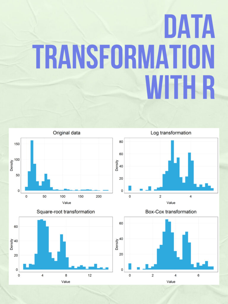
  1. Visualize the data: Once the data is cleaned and prepared, you can start visualizing it using Matplotlib and Seaborn. Matplotlib provides basic visualization functions like plot(), scatter(), hist(), etc., while Seaborn provides more advanced functions for statistical data visualization, such as distplot(), boxplot(), heatmap(), etc. Here’s an example of creating a histogram of age distribution using Seaborn:
sns.distplot(data['age'], bins=10)
plt.title('Age Distribution')
plt.xlabel('Age')
plt.ylabel('Density')
plt.show()

These are the basic steps of course, there are many more advanced techniques and libraries available, depending on your specific needs and goals.

Download(PDF)

Line graph with R

A line graph is a type of chart used to display data as a series of points connected by lines. It is commonly used to show trends over time or to compare multiple data sets. Line graphs are useful for visualizing data that changes continuously over time, such as stock prices, weather patterns, or population growth. They can also be used to compare multiple data sets, such as the performance of different companies in a particular industry. To create a line graph in R, you can use the built-in plot() function or the more powerful ggplot2 library. Here is an example of how to create a line graph using ggplot2.

Line graph with R
Line graph with R

First, let’s create a sample data frame with some random values:

# Create sample data frame
x <- 1:10
y <- c(3, 5, 6, 8, 10, 12, 11, 9, 7, 4)
df <- data.frame(x, y)

Next, we’ll use ggplot() to create a plot object, and then add a geom_line() layer to draw the line:

# Load ggplot2 library
library(ggplot2)

# Create plot object
p <- ggplot(df, aes(x, y))

# Add line layer
p + geom_line()

This will create a basic line graph with the x values on the x-axis and the y values on the y-axis. You can customize the appearance of the graph by adding additional layers or modifying the ggplot() object. For example, you can add axis labels and a title:

# Add axis labels and title
p + geom_line() + 
  labs(x = "X-axis label", y = "Y-axis label", title = "Title of the graph")

You can also modify the line color and thickness using the color and size arguments of geom_line():

# Change line color and thickness
p + geom_line(color = "red", size = 2) +
  labs(x = "X-axis label", y = "Y-axis label", title = "Title of the graph")

These are just a few examples of the many customization options available in ggplot2.

Download(PDF)

Data Structures and Algorithms with Python

Data structures and algorithms are fundamental concepts in computer science and software engineering. They help us solve problems more efficiently by organizing and manipulating data in a way that allows for faster retrieval and processing. Python is a popular programming language that is widely used for data analysis, scientific computing, web development, and many other applications. It provides a rich set of built-in data structures and libraries that make it easy to implement common algorithms and data structures.

Data Structures and Algorithms with Python

Some of the commonly used data structures in Python include lists, tuples, sets, and dictionaries. Lists are mutable sequences of elements, tuples are immutable sequences, sets are unordered collections of unique elements, and dictionaries are mappings between keys and values.

There are also several libraries in Python that provide more advanced data structures and algorithms, such as NumPy, Pandas, and Scikit-learn for data analysis and machine learning, and NetworkX for graph algorithms.

When it comes to algorithms, Python provides a rich set of built-in functions and libraries that make it easy to implement common algorithms, such as sorting, searching, and graph traversal. Some of the popular algorithms that are commonly implemented in Python include binary search, quicksort, mergesort, and breadth-first search.

To master data structures and algorithms with Python, it is important to have a good understanding of the fundamental concepts, as well as the specific features and libraries provided by the language. It is also helpful to practice implementing algorithms and data structures in Python and to study examples and tutorials from experienced programmers and online resources.

Download(PDF)

Statistics and Data Analysis for Financial Engineering

Statistics and data analysis are essential skills for financial engineering, as they provide the foundation for modeling and analyzing financial data. R is a popular programming language for data analysis and statistical modeling, and it has numerous packages that are well-suited for financial engineering applications. Here are some key areas where statistics and data analysis can be applied in financial engineering using R:

Statistics and Data Analysis for Financial Engineering

Risk Analysis: Financial engineers use statistical methods to estimate the likelihood of different types of risks, such as market risk, credit risk, and operational risk. R has several packages like “Risk” and “fBasics” that can be used to perform different types of risk analysis.

Time Series Analysis: Financial time series data typically exhibit patterns such as trends, seasonality, and autocorrelation. R has several packages like “tseries” and “forecast” that are specifically designed for analyzing time series data.

Portfolio Optimization: Financial engineers use statistical methods to optimize investment portfolios by balancing risk and return. R has several packages like “PortfolioAnalytics” and “quantmod” that can be used to perform portfolio optimization.

Monte Carlo Simulation: Monte Carlo simulation is a powerful statistical technique used to model complex systems and estimate probabilities. In finance, Monte Carlo simulation is used to estimate the value of financial derivatives and to simulate the behavior of financial markets. R has several packages like “mc2d” and “MCMCpack” that can be used for Monte Carlo simulation.

Data Visualization: Data visualization is an important part of data analysis in financial engineering. R has several packages like “ggplot2” and “lattice” that can be used to create visualizations of financial data.

Download(PDF)

Create an area graph with R

Create an area graph with R: Area graphs are a great way to visualize data over time, especially when you want to see how different data sets contribute to an overall trend. In this tutorial, we will be using R programming to create an area graph using the ggplot2 library.

Create an area graph with R

First, we need to install and load the ggplot2 library:

install.packages("ggplot2")
library(ggplot2)

Next, we need some data to work with. We will be using the built-in economics data set that comes with R, which contains data on the US economy from 1967 to 2015:

data(economics)

To create an area graph with ggplot2, we first need to prepare the data by converting it from a wide format to a long format using the gather function from the tidyr library:

library(tidyr)
economics_long <- gather(economics, key = "variable", value = "value", -date)

This code creates a new data frame called economics_long that has three columns: date, variable, and value. The date column contains the dates from the original economics data set, the variable column contains the names of the different economic indicators, and the value column contains the corresponding values for each indicator on each date.

Now that we have our data in the right format, we can create our area graph using ggplot2:

ggplot(economics_long, aes(x = date, y = value, fill = variable)) +
  geom_area()

This code creates a new ggplot object that uses the economics_long data frame as its data source. The aes function is used to specify the variables to be plotted: the date column on the x-axis, the value column on the y-axis, and the variable column for the fill color of the areas. The geom_area function is used actually to create the area graph.

By default, ggplot2 stacks the areas on top of each other, but we can change this by adding the position = "identity" argument to the geom_area function

ggplot(economics_long, aes(x = date, y = value, fill = variable)) +   geom_area(position = "identity") 

This code creates the same area graph as before, but with the area’s side by side instead of stacked.

We can also customize the graph’s appearance by adding labels, adjusting the color scheme, and so on. Here’s an example:

ggplot(economics_long, aes(x = date, y = value, fill = variable)) +
  geom_area(position = "identity", alpha = 0.7, color = "white") +
  scale_fill_manual(values = c("#FF5733", "#C70039", "#900C3F", "#581845")) +
  labs(title = "US Economic Indicators",
       subtitle = "1967-2015",
       x = "Year",
       y = "Value",
       fill = "Indicator") +
  theme_minimal()

This code creates an area graph with a reduced alpha value to add transparency, a white border for each area, and a custom color scheme using the scale_fill_manual function. We also added a title and subtitle, labels for the x- and y-axes, and a legend label using the labs function. Finally, we applied the theme_minimal theme to give the graph a clean, modern look.

ANOVA in R

ANOVA (Analysis of Variance) is a statistical technique used to determine whether there are any significant differences between the means of two or more groups. R is a powerful programming language used for statistical analysis, and it includes several functions for conducting ANOVA. In this article, we will discuss how to perform ANOVA in R.

ANOVA in R
ANOVA in R
  1. Install Required Packages To perform ANOVA in R, you need to install two packages: “car” and “multcomp”. You can install these packages using the following command:
install.packages("car")
install.packages("multcomp")
  1. Load the Required Libraries After installing the required packages, you need to load them into R using the following command:
library(car)
library(multcomp)
  1. Prepare the Data Before performing ANOVA, you need to prepare your data. The data should be organized in a way that allows you to compare the means of different groups. The data can be in the form of a CSV file, a spreadsheet, or a data frame in R.
  2. Conduct ANOVA Once your data is prepared, you can conduct ANOVA using the aov() function in R. The aov() function takes two arguments: the first argument is the formula that specifies the variables and their interactions, and the second argument is the data frame that contains the data.

For example, suppose we have a dataset called “mydata” that contains three variables: “group”, “score1”, and “score2”. The “group” variable has three levels (A, B, and C), and the “score1” and “score2” variables contain the scores of the participants in each group. To perform ANOVA, we can use the following code:

mydata <- read.csv("data.csv")
mydata$group <- factor(mydata$group)
fit <- aov(cbind(score1, score2) ~ group, data=mydata)

In this example, we first load the data from a CSV file called “data.csv”. We then convert the “group” variable into a factor using the factor() function. Finally, we use the aov() function to conduct ANOVA on the “score1” and “score2” variables, with the “group” variable as the factor.

  1. Check for Significant Differences After conducting ANOVA, you need to check whether there are any significant differences between the means of the groups. You can do this using the summary() function in R.
summary(fit)

The summary() function will provide you with the F-statistic, the degrees of freedom, and the p-value for each variable in the model. The p-value indicates the significance level of the variable, and a p-value less than 0.05 indicates that the variable is significant.

  1. Post-hoc Analysis If ANOVA indicates that there are significant differences between the means of the groups, you can perform post-hoc analysis to determine which groups are significantly different from each other. You can do this using the TukeyHSD() function in R.
TukeyHSD(fit)

The TukeyHSD() function will perform Tukey’s Honest Significant Difference (HSD) test, which is a post-hoc test that compares all pairs of groups and determines which pairs are significantly different from each other. The output of the TukeyHSD() function will provide you with the p-value and the confidence interval for each pair of groups.

Download(PDF)


Errors in R and how to fix them

R is a powerful programming language for data analysis, but errors are inevitable. By understanding the common errors and how to fix them, you can write more robust and efficient code. In this article, we will look at the top errors in R and how to fix them.

Errors in R and how to fix them
  1. Syntax Errors Syntax errors are the most common errors in R. These errors occur when the code is not written correctly. It could be a missing comma, a misplaced parenthesis, or a misspelled function. R will show an error message with the line number where the error occurred. To fix the error, go to that line and correct the syntax.
  2. Object Not Found Errors This error occurs when you try to access an object that doesn’t exist. It could be a variable or a function that has not been defined. To fix this error, check if the object is defined or if there is a typo in the object name. You can also check if the object is in the correct environment.
  3. Data Type Errors R is a strongly typed language, which means that each variable has a specific data type. Data type errors occur when you try to assign a value of one data type to a variable of a different data type. For example, trying to assign a string to a numeric variable. To fix this error, make sure that the data type of the variable matches the data type of the value.
  4. Out of Memory Errors, R uses memory to store data and variables. If you try to load a large dataset or perform a computation that requires more memory than is available, you will get an out-of-memory error. To fix this error, try freeing up memory by removing unnecessary objects or using more efficient code. You can also increase the memory available to R by using the “memory.limit()” function.
  5. Package Not Found Errors R has a vast collection of packages that extend its functionality. If you try to use a package that is not installed, you will get a package not found error. To fix this error, install the required package using the “install.packages()” function. You can also check if the package is spelled correctly.
  6. Infinite and Missing Values In R, missing values are represented by NA, and infinite values are represented by Inf. If you perform a computation that results in an infinite or missing value, you will get an error. To fix this error, you can remove the missing or infinite values using the “na.omit()” and “is.finite()” functions.
  7. Unintended Loops Loops are powerful constructs in R, but they can cause errors if not used correctly. Unintended loops occur when a loop is not correctly structured, leading to an infinite loop or a loop that never executes. To fix this error, check the loop structure and ensure that it terminates when it should.

Data transformation with R

Data transformation is a crucial step in data analysis, and R provides many powerful tools for transforming and manipulating data. Here is an example of data transformation using R: Suppose you have a dataset called “mydata” that contains information about some customers, including their name, age, gender, and income. Here is a sample of what the data might look like:

Data transformation with R
   name  age gender income
1   Bob   25      M  50000
2 Alice   30      F  60000
3   Tom   35      M  70000
4   Sue   40      F  80000

Now, let’s say you want to perform some data transformation on this dataset. Here are some common data transformations that you can do with R:

  1. Subset the data:

You can select a subset of the data based on some criteria using the subset() function. For example, you can select only the customers who are over 30 years old:

mydata_subset <- subset(mydata, age > 30)

This will create a new dataset called “mydata_subset” that contains only the rows where age is greater than 30.

  1. Rename columns:

You can rename the columns in the dataset using the colnames() function. For example, you can rename the “gender” column to “sex”:

colnames(mydata)[3] <- "sex"

This will rename the third column (which is the “gender” column) to “sex”.

  1. Reorder columns:

You can reorder the columns in the dataset using the select() function from the dplyr package. For example, you can move the “income” column to the front of the dataset:

library(dplyr)
mydata_new <- select(mydata, income, everything())

This will create a new dataset called “mydata_new” that has the “income” column as the first column, followed by the other columns in the original dataset.

  1. Create new columns:

You can create new columns in the dataset based on some calculation or function using the mutate() function from the dplyr package. For example, you can create a new column called “income_log” that contains the logarithm of the “income” column:

mydata_new <- mutate(mydata, income_log = log(income))

This will create a new dataset called “mydata_new” that has a new column called “income_log” containing the logarithm of the “income” column.

  1. Group and summarize data:

You can group the data based on some variable and summarize the data using the group_by() and summarize() functions from the dplyr package. For example, you can group the data by “sex” and calculate the average income for each sex:

mydata_summary <- mydata %>%
  group_by(sex) %>%
  summarize(avg_income = mean(income))

This will create a new dataset called “mydata_summary” that has two rows (one for each sex) and one column called “avg_income” containing the average income for each sex.

Download(PDF)

Statistical Learning with Math and R

Statistical Learning with Math and R: Statistical learning is an essential tool for data analysis and machine learning. It involves using mathematical methods and programming languages like R to analyze and model data. In this article, we will discuss statistical learning and its applications in data science.

Statistical Learning with Math and R

What is statistical learning?

Statistical learning is a field of study that focuses on building models to make predictions or decisions based on data. It involves using statistical and mathematical techniques to extract insights from data. Statistical learning models can be used to understand relationships between variables, predict outcomes, and make decisions.

The goal of statistical learning is to find patterns and relationships within data that can be used to make predictions. It can be supervised or unsupervised. The model is trained using labeled data in supervised learning, where the outcome variable is known. In unsupervised learning, the model is trained using unlabeled data, and the goal is to discover hidden patterns or structures within the data.

Mathematics in Statistical learning

Mathematics is a fundamental aspect of statistical learning. It provides the necessary tools to model and analyze data. Linear algebra, calculus, probability theory, and optimization are all essential mathematical concepts used in statistical learning.

Linear algebra is used to represent data in a structured way, such as vectors and matrices. It is also used to solve systems of equations and perform operations such as matrix multiplication and matrix inversion.

Calculus is used to optimize models and find the best parameters that fit the data. It is used to find the maximum or minimum of a function, which can be used to optimize model parameters.

Probability theory is used to understand the uncertainty in data and make predictions based on probabilities. It is used to model random variables and distributions, essential for building statistical models.

Optimization is used to find the best parameters for a model that fit the data. It involves finding the minimum or maximum of a function, which can be done using calculus.

R in Statistical learning

R is a programming language and environment that is widely used for statistical computing and graphics. It provides a range of tools and packages for data analysis, visualization, and modeling. R is an open-source language, which means that it is free to use, and it has a large community of users who contribute to its development.

R provides a range of packages for statistical learning, such as caret, glmnet, randomForest, and xgboost. These packages provide tools for building and evaluating models, as well as tools for preprocessing data and performing feature selection.

R also provides a range of visualization tools, such as ggplot2, which can be used to visualize data and model outputs. Visualization is an essential aspect of statistical learning because it helps to understand the relationships between variables and the performance of models.

Download(PDF)

Math And Python Statistical Learning

Statistical learning is a branch of statistics that deals with modeling and analyzing data using various mathematical and computational tools. It involves understanding the underlying patterns and relationships within the data and using them to make predictions and informed decisions. Python is a popular programming language used for statistical learning, as it offers a wide range of powerful libraries and tools for data analysis, visualization, and machine learning.

Math And Python Statistical Learning

To get started with statistical learning using math and Python, here are some key concepts and tools to consider:

  1. Probability and statistics: A solid foundation in probability theory and statistics is essential for statistical learning. This includes understanding concepts such as probability distributions, hypothesis testing, regression analysis, and Bayesian inference.
  2. Linear algebra: Linear algebra is a fundamental mathematical concept that underpins many statistical learning algorithms. Understanding concepts such as vectors, matrices, and eigenvectors can help with tasks such as data preprocessing, dimensionality reduction, and optimization.
  3. Python libraries: Python has a wealth of libraries and tools for statistical learning, including NumPy for numerical computing, pandas for data manipulation, matplotlib and seaborn for data visualization, and scikit-learn for machine learning algorithms.
  4. Data preprocessing: Before applying statistical learning algorithms, data must be preprocessed and cleaned. This includes tasks such as removing missing values, scaling features, and handling categorical variables.
  5. Machine learning algorithms: There are many machine learning algorithms that can be used for statistical learning, including linear regression, logistic regression, decision trees, random forests, support vector machines, and neural networks. Each algorithm has its strengths and weaknesses, and choosing the right one depends on the specific task and data at hand.

Overall, statistical learning with math and Python requires a combination of mathematical knowledge, programming skills, and domain expertise. With the right tools and understanding, you can use statistical learning to gain insights from data and make more informed decisions.

Download(PDF)