PYOFLIFE

Learn the Central Limit Theorem in R: The Central Limit Theorem (CLT) is a fundamental concept in statistics that states that if you have a large sample size from any population with a finite mean and variance, then the sampling distribution of the mean will be approximately normal regardless of the shape of the original population distribution. In this tutorial, I will walk you through how to simulate the CLT using R step by step.

Step 1: Load Required Libraries We will be using the libraries “ggplot2” and “gridExtra” for this tutorial. So, we need to install and load them using the following code:

install.packages("ggplot2")
install.packages("gridExtra")

library(ggplot2)
library(gridExtra)

Step 2: Generate Data Let’s generate some data for this example. We will use the exponential distribution as our population distribution. The exponential distribution is a continuous probability distribution that describes the time between events in a Poisson process. It has a single parameter, which is the rate parameter.

set.seed(123) # for reproducibility
population <- rexp(1000, rate = 1)

Here, we generated 1000 observations from an exponential distribution with a rate parameter of 1.

Step 3: Simulate Sampling Distribution of Means To simulate the CLT, we will take random samples of size n from the population and calculate the mean. We will repeat this process 1000 times and store the means in a vector.

n <- 10 # sample size
num.simulations <- 1000 # number of simulations

sample.means <- replicate(num.simulations, mean(sample(population, n)))

Here, we took random samples of size 10 from the population and calculated the mean. We repeated this process 1000 times and stored the means in the vector “sample.means”.

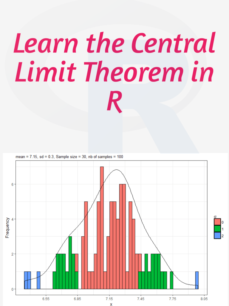
Step 4: Visualize Sampling Distribution of Means Now, we can visualize the sampling distribution of means using a histogram.

# histogram of sample means
ggplot(data.frame(sample.means), aes(x = sample.means)) + 
  geom_histogram(aes(y = ..density..), color = "black", fill = "white", binwidth = 0.2) +
  stat_function(fun = dnorm, args = list(mean = mean(population), sd = sd(population)/sqrt(n)), color = "red", size = 1) +
  ggtitle(paste("Sampling Distribution of Means (n = ", n, ")", sep = "")) +
  xlab("Sample Means") +
  ylab("Density")

In this code, we created a histogram of the sample means and added a red line for the theoretical normal distribution with the same mean and standard deviation as the sampling distribution of means. We also added a title and axis labels to the plot.

Step 5: Repeat with Different Sample Sizes Finally, we can repeat this process for different sample sizes and visualize the results using a grid of plots.

# function to simulate CLT and create plot
plot_CLT <- function(n) {
  sample.means <- replicate(num.simulations, mean(sample(population, n)))
  
  plot <- ggplot(data.frame(sample.means), aes(x = sample.means)) + 
    geom_histogram(aes(y = ..density..), color = "black", fill = "white", binwidth = 0.2) +
    stat_function(fun = dnorm, args = list(mean = mean(population), sd = sd(population)/sqrt(n)), color = "red", size = 1) +
    ggtitle(p

R is a powerful programming language used for data analysis and statistical computing. However, writing efficient and effective R code can be challenging, especially for those who are new to the language. In this article, we will discuss five tips to improve your R code and make it more readable, efficient, and reliable.

1. Use vectorization

Vectorization is the process of performing operations on entire vectors instead of individual elements. This technique can significantly improve the performance of your code by reducing the number of loops required. For example, instead of using a for loop to add two vectors element-wise, you can use the “+” operator to add the vectors directly.

Here’s an example:

# Using a for loop
x <- 1:1000
y <- 1:1000
z <- numeric(length(x))

for (i in 1:length(x)) {
  z[i] <- x[i] + y[i]
}

# Using vectorization
x <- 1:1000
y <- 1:1000
z <- x + y

2. Avoid global variables

Using global variables can make your code more difficult to debug and maintain, especially when dealing with large programs. It’s best to use local variables instead, which are created and used within a function. This approach can also help avoid naming conflicts between different parts of your code.

Here’s an example:

# Using global variables
x <- 10

my_function <- function() {
  y <- x + 5
  return(y)
}

# Using local variables
my_function <- function(x) {
  y <- x + 5
  return(y)
}

result <- my_function(10)

3. Use appropriate data structures

Choosing the appropriate data structure can make a significant difference in the performance of your code. For example, using a matrix instead of a data frame can be faster for numerical operations, while using a list can be more flexible for storing different types of objects.

Here’s an example:

# Using a matrix
x <- matrix(1:1000000, nrow = 1000)
row_sums <- apply(x, 1, sum)

# Using a data frame
x <- data.frame(matrix(1:1000000, nrow = 1000))
row_sums <- apply(x, 1, sum)

# Using a list
my_list <- list(a = 1, b = "hello", c = TRUE)

4. Write readable code

Writing readable code can make it easier for others to understand your code and for you to maintain it in the future. Some best practices for writing readable code include using descriptive variable names, writing comments to explain complex code, and formatting your code consistently.

Here’s an example:

# Writing readable code
x <- c(1, 2, 3, 4, 5) # Create a vector of numbers
y <- sum(x) # Calculate the sum of the vector

5. Use functions from packages

R has a vast library of packages that provide pre-built functions for a wide range of tasks. Using functions from these packages can save you time and improve the reliability of your code, as these functions have often been thoroughly tested and optimized.

Here’s an example:

# Using a function from a package
library(dplyr)

x <- data.frame(a = c(1, 2, 3), b = c(4, 5, 6))
y <- select(x, a) # Select the 'a' column of the data frame

These five tips can help you improve your R code and make it more efficient, readable, and reliable.

A box plot is a graphical representation of a dataset that displays the distribution of data through five summary statistics: the minimum value, the first quartile (25th percentile), the median (50th percentile), the third quartile (75th percentile), and the maximum value. The box in the plot represents the middle 50% of the data (between the first and third quartiles), while the whiskers extend from the box to show the range of the data, excluding any outliers. Outliers are represented by dots or asterisks outside the whiskers. Box plots are useful for quickly visualizing the spread, skewness, and outliers of a dataset. They are commonly used in statistical analysis, especially for comparing distributions between different groups or variables.

To make a boxplot in R, you can use the boxplot() function, which is a built-in function in R. Here’s an example code:

# Create a vector of data
data <- c(10, 20, 15, 30, 25, 35, 40, 50)

# Create a boxplot of the data
boxplot(data)

In the above example, we first create a vector of data called data. Then we use the boxplot() function to create a boxplot of the data.

You can customize the boxplot by adding different parameters to the boxplot() function. Here are some examples:

• Adding a title to the plot:

boxplot(data, main="Boxplot of Data")

• Changing the x-axis label:

boxplot(data, xlab="Data")

• Changing the color of the box and whiskers:

boxplot(data, col="blue")

• Creating a horizontal boxplot:

boxplot(data, horizontal=TRUE)

These are just a few examples of how you can customize the boxplot in R. You can find more information about the boxplot() function and its parameters in the R documentation.

Read more: How to Create a Population Pyramid in R?

An age-sex pyramid is also known as a population pyramid. Using it, we can visualize the distribution of a population by age group and gender. In general, it resembles a pyramid. Females are represented on the right of the population pyramid, while males are typically depicted on the left. Based on the number or percentage of men and women in a particular population, this data visualization method can be used to visualize that population’s age. Creating a population pyramid in R is a common data analysis and visualization task. Here are the steps to create a population pyramid in R:

Download:

Step 1: Install and load necessary packages Before starting to create a population pyramid, we need to install and load the ggplot2 and dplyr packages. These packages are used for data visualization and data manipulation, respectively.

install.packages("ggplot2")
install.packages("dplyr")

library(ggplot2)
library(dplyr)

Step 2: Load the Data To create a population pyramid, we need data on the age and sex distribution of the population. We can use the built-in “midwest” dataset from ggplot2 package as an example.

data(midwest)

Step 3: Data Wrangling Next, we need to prepare the data for the population pyramid visualization. We will use the dplyr package to manipulate the data.

midwest <- midwest %>%
  select(county, state, Poptotal, popdensity, percwhite, percblack, percamericanindian, percasian, perchispanic, percother, medianage, medianhousevalue, medianincome, region, division) %>%
  filter(!is.na(Poptotal), !is.na(medianage)) %>%
  mutate_at(vars(percwhite:percother), ~replace_na(., 0))

Step 4: Create the Population Pyramid Now, we can create the population pyramid using the ggplot2 package.

ggplot(midwest, aes(x = medianage, y = Poptotal, fill = factor(ifelse(medianage < 37.5, "Male", "Female")))) +
  geom_bar(stat = "identity", position = "identity") +
  scale_fill_manual(values = c("#619CFF", "#FF6161")) +
  labs(title = "Population Pyramid", x = "Median Age", y = "Population", fill = "") +
  coord_flip()

This will create a population pyramid in R, showing the age and sex distribution of the population.

The above example is just a sample, and you can use your own data to create the population pyramid in R.

There are several ways to create a dashboard in R, but one of the most popular and powerful options is to use the Shiny package. Shiny allows you to build interactive web applications directly from R code, including data visualization and analysis. Here are the general steps to creating a dashboard in R using Shiny:

1. Install and load the Shiny package:

install.packages("shiny")
library(shiny)

2. Load your data: You can use any data source that you like, but it’s important to make sure that the data is in a format that can be used by Shiny.
3. Create a user interface (UI): This is where you define what the user will see and interact with in your dashboard. You can use Shiny’s built-in UI elements (such as sliders, drop-down menus, and text boxes) or create your own custom UI elements using HTML, CSS, and JavaScript.
4. Create a server function: This is where you define the logic and calculations that will power your dashboard. You can use any R code you like, including data manipulation and analysis functions.
5. Combine the UI and server: Use the shinyApp() function to combine the UI and server functions into a complete Shiny application.
6. Deploy your dashboard: You can deploy your Shiny dashboard to a variety of platforms, including shinyapps.io and your own web server.

Here’s a basic example of a Shiny dashboard that displays a histogram of a dataset:

# Load the Shiny package
library(shiny)

# Load the dataset
data(mtcars)

# Define the UI
ui <- fluidPage(
  titlePanel("MTCars Histogram"),
  sidebarLayout(
    sidebarPanel(
      sliderInput("bins", "Number of bins:", min = 1, max = 50, value = 30)
    ),
    mainPanel(
      plotOutput("histogram")
    )
  )
)

# Define the server
server <- function(input, output) {
  output$histogram <- renderPlot({
    bins <- seq(min(mtcars$mpg), max(mtcars$mpg), length.out = input$bins + 1)
    hist(mtcars$mpg, breaks = bins, col = "blue", main = "MTCars Histogram")
  })
}

# Combine the UI and server
shinyApp(ui = ui, server = server)

This code creates a Shiny app with a slider that allows the user to control the number of bins in a histogram of the mpg column of the mtcars dataset. When the user moves the slider, the histogram is updated in real-time. You can customize this example and add more elements to create a full dashboard with multiple charts, tables, and other interactive features.

Download:

A confidence interval is a range of values that provides a plausible range of values for an unknown population parameter, based on a sample from that population. The confidence interval is expressed as a percentage, such as 95% or 99%, which represents the level of confidence you have that the true population parameter falls within the interval. For example, if you calculate a 95% confidence interval for the average height of students in the school, you can say with 95% confidence that the true average height falls within that range of values. Calculating confidence intervals using R is relatively simple. Here’s a general process you can follow:

1. Load your data into R. You can do this by typing the name of your data file, followed by the read.table() function, like this: mydata <- read.table("myfile.txt", header=TRUE). This assumes that your data is in a tab-delimited text file with headers.
2. Calculate the sample mean and standard deviation. You can use the mean() and sd() functions in R to do this, like this: mymean <- mean(mydata$myvariable) and mysd <- sd(mydata$myvariable). Replace “myvariable” with the name of the variable in your data that you want to calculate the confidence interval for.
3. Determine the sample size. You can use the nrow() function in R to get the number of rows (i.e., observations) in your data, like this: mysize <- nrow(mydata).
4. Choose a confidence level. You’ll need to decide on a confidence level for your confidence interval. For example, you might choose 95%, which is a common level of confidence.
5. Calculate the confidence interval. You can use the t.test() function in R to calculate the confidence interval, like this: myci <- t.test(mydata$myvariable, conf.level=0.95)$conf.int. This will give you a 95% confidence interval for the mean of your variable.
6. Print or save the confidence interval. You can use the print() function to print the confidence interval to the console, like this: print(myci). Or you can save it to a variable and use it later in your code, like this: myci <- t.test(mydata$myvariable, conf.level=0.95)$conf.int.

Keep in mind that the exact method of calculating the confidence interval may vary depending on the type of data you’re working with and the statistical test you’re using. But the general process outlined above should give you a good starting point for calculating confidence intervals in R.

Related post: ANOVA in R

Download(PDF)