Books

Econometrics is a branch of economics that uses statistical and mathematical methods to analyze economic data. It is an important tool for economists and policymakers to make informed decisions about economic policies and forecast economic outcomes. R is a programming language widely used in econometrics to analyze, visualize, and interpret data. In this article, we will provide an introduction to econometrics with R. We will discuss the basic concepts of econometrics and how R can be used to apply these concepts.

What is Econometrics?

Econometrics is the application of statistical methods to economic data to test economic theories and forecast economic outcomes. It is used to estimate the relationships between economic variables, such as price and quantity, income and expenditure, and interest rates and investment. Econometrics uses statistical models to describe the relationships between these variables and to make predictions about future economic behavior.

Econometrics involves three steps:

1. Specification: This involves defining the economic theory and the variables that will be used to test it.
2. Estimation: This involves estimating the parameters of the model using statistical methods.
3. Evaluation: This involves testing the validity of the model and the accuracy of the predictions.

R and Econometrics

R is a popular programming language used in econometrics because of its versatility and its ability to handle large and complex datasets. R provides a wide range of functions for econometric analysis, including linear regression, time-series analysis, panel data analysis, and non-parametric analysis.

R also provides a wide range of visualization tools, including graphs, charts, and tables, to help economists and policymakers understand economic data and make informed decisions.

Using R for Econometric Analysis

To use R for econometric analysis, you will need to install the relevant packages for your analysis. There are several packages available for econometric analysis, including:

1. plm: This package is used for panel data analysis.
2. lmtest: This package is used for hypothesis testing of linear regression models.
3. tsDyn: This package is used for time-series analysis.
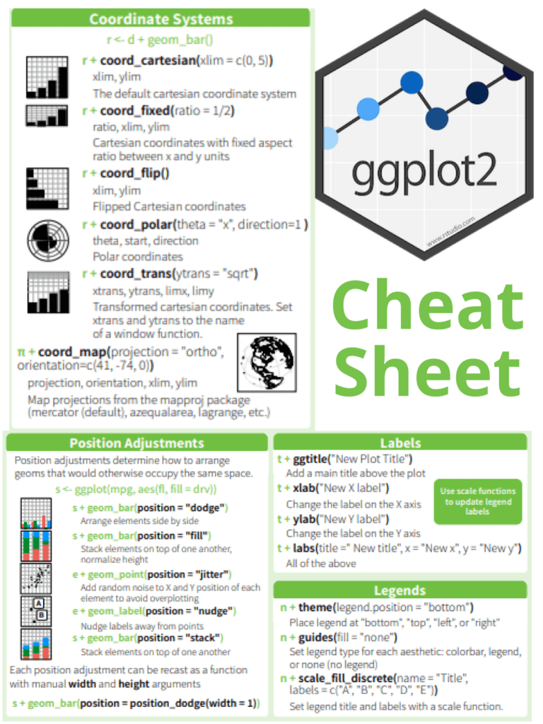
4. ggplot2: This package is used for data visualization.

Once you have installed the relevant packages, you can start using R for econometric analysis. Here are some basic steps:

1. Load the data: You can load data into R using various methods, including CSV files, Excel files, or SQL databases.
2. Clean and preprocess the data: This involves removing missing values, and outliers, and transforming the data if necessary.
3. Model specification: This involves defining the economic theory and the variables that will be used to test it.
4. Estimation: This involves estimating the parameters of the model using statistical methods.
5. Evaluation: This involves testing the validity of the model and the accuracy of the predictions.
6. Visualization: This involves creating graphs, charts, and tables to help understand and communicate the results of the analysis.

Download(PDF)

Geocomputation with R is a powerful tool for spatial analysis that has gained widespread popularity in recent years. R is a free and open-source programming language that provides a comprehensive platform for geocomputation, which combines statistical and computational methods with geographic information systems (GIS) to analyze spatial data.

R provides a wide range of functions and packages for geocomputation, including mapping, geostatistics, spatial data manipulation, and spatial analysis. It also offers access to a wealth of data sources, including remote sensing data, census data, and environmental data, among others.

One of the key advantages is its ability to handle large and complex spatial datasets. R provides an efficient and flexible framework for data manipulation and processing, allowing users to work with datasets that would be too large or too complex to analyze using traditional GIS software.

Another advantage of geocomputation with R is its ability to integrate with other data analysis tools. R provides easy integration with other programming languages, such as Python and SQL, as well as with popular data analysis tools like Excel and Tableau. This makes it easy for users to import and export data, as well as to share results with others.

Geocomputation with R is also highly customizable, allowing users to tailor their analysis to their specific needs. R provides a wide range of packages and functions, as well as the ability to create custom functions and scripts. This flexibility enables users to adapt their analysis to different types of spatial data, as well as to different research questions and hypotheses.

The popularity of geocomputation with R has led to the development of a vibrant and supportive community of users and developers. The R spatial community includes a wide range of individuals, from academics and researchers to practitioners and enthusiasts. This community provides a rich source of knowledge and support, as well as a forum for sharing ideas and best practices.

Geocomputation with R has numerous applications across a range of disciplines, including geography, ecology, epidemiology, and urban planning, among others. Some of the key applications of geocomputation with R include:

• Mapping and visualization of spatial data
• Spatial analysis of environmental and ecological data
• Spatial modeling and prediction
• Spatial optimization and decision-making
• Geostatistics and spatial interpolation

Geocomputation with R is a powerful tool for spatial analysis that provides a flexible and efficient platform for handling large and complex spatial datasets. Its ability to integrate with other data analysis tools, as well as its highly customizable nature, make it a popular choice for researchers and practitioners across a range of disciplines. With a supportive and active community of users and developers, geocomputation with R is poised to remain a leading tool for spatial analysis in the years to come.

Read More: Geographic Data Science with R

Download(PDF)

Geographic Data Science is an emerging field that combines spatial analysis, statistical modeling, and data visualization techniques to explore patterns and relationships within geographic data. With the advent of open-source software and programming languages like Python, it has become easier than ever before to work with large datasets and create dynamic visualizations that reveal complex patterns in geographic data.

Python is a popular programming language for Geographic Data Science due to its versatility, ease of use, and wide range of powerful libraries such as geopandas, matplotlib, and seaborn. These libraries enable users to easily manipulate, visualize and analyze geographic data.

The geopandas library is particularly useful for working with geospatial data as it provides an easy way to read, write, and manipulate geographic data in a variety of formats, such as shapefiles and GeoJSON files. It also allows users to perform spatial operations such as overlaying polygons, buffering points, and calculating distances.

Matplotlib and seaborn are two popular libraries for data visualization in Python. Matplotlib provides a wide range of customizable plots such as scatterplots, histograms, and heatmaps. Seaborn, on the other hand, provides a higher-level interface for creating more complex visualizations such as heatmaps with annotations and faceted plots.

Another important library for Geographic Data Science in Python is scikit-learn. It provides a range of machine learning algorithms that can be applied to geographic data, such as clustering and classification. For instance, clustering algorithms can be used to group similar locations together based on their features, while classification algorithms can be used to predict the land use of a given area based on its features.

With these libraries, Geographic Data Science with Python can be applied to a wide range of applications. For instance, it can be used to analyze environmental data, such as air pollution levels, and identify hotspots where pollution is most severe. It can also be used to analyze demographic data and identify patterns of inequality or segregation within a city.

Learn More: Geographic Data Science with R

Download(PDF)

Time series analysis is a statistical technique used to analyze and interpret data that varies over time. Time series data is common in many fields, including economics, finance, engineering, and environmental science. In this response, we will discuss the basics of time series analysis and its applications in R.

Basics of Time Series Analysis

A time series is a collection of observations made over time. The data can be in continuous or discrete time intervals. Time series data can be analyzed to identify patterns, trends, and relationships between variables. Some common characteristics of time series data include:

• Trend: The overall direction of the data over time.
• Seasonality: Repeating patterns over fixed time intervals.
• Cyclicity: Repeating patterns over variable time intervals.
• Autocorrelation: Correlation between observations at different time points.

Time series analysis involves several steps, including data visualization, identifying trends and patterns, fitting models to the data, and making forecasts. There are several statistical techniques used in time series analysis, including autoregressive integrated moving average (ARIMA) models, exponential smoothing models, and spectral analysis.

Applications in R

R is a powerful programming language for statistical computing and graphics that is widely used for time series analysis. The forecast package in R provides several functions for time series analysis, including auto.arima for automatically selecting an appropriate ARIMA model, ets for exponential smoothing models, and acf and pacf for autocorrelation and partial autocorrelation plots.

To get started with time series analysis in R, you can use the ts function to create a time series object from a vector or matrix of data. You can then plot the data using the plot function, and use the various functions in the forecast package to fit models and make forecasts.

Here is an example of fitting an ARIMA model to time series data:

# Load the data
data <- read.csv("data.csv")

# Convert data to time series object
ts_data <- ts(data$Sales, start = c(2010, 1), frequency = 12)

# Fit an ARIMA model
model <- auto.arima(ts_data)

# Make a forecast for the next 12 months
forecast <- forecast(model, h = 12)

# Plot the forecast
plot(forecast)

In this example, we first load the data from a CSV file and convert it to a time series object using the ts function. We then fit an ARIMA model to the data using the auto.arima function, which automatically selects an appropriate model based on the data. We make a forecast for the next 12 months using the forecast function, and plot the forecast using the plot function.

Overall, R provides a powerful and flexible environment for time series analysis, with many built-in functions and packages for working with time series data.

Learn More: Statistics and Data Analysis for Financial Engineering

Download(PDF)

If you’re an aspiring data scientist, chances are you’ve come across ggplot2, a powerful data visualization package in R. However, with its wide range of options and functionalities, it can be overwhelming to memorize all the different commands and syntax. Fortunately, ggplot2 has a handy cheat sheet that summarizes all the basic elements and syntax, making it easier for you to create beautiful visualizations.

The ggplot2 cheat sheet covers all the key components of the package, including data layers, scales, aesthetics, and geometries. It’s a comprehensive guide that can help you quickly create complex visualizations without having to remember all the details of the package’s syntax.

Here are some of the key elements you’ll find on the ggplot2 cheat sheet:

• Data layers: The data layer is the foundation of any ggplot2 visualization. It’s where you specify the dataset you want to use and the variables you want to visualize. The cheat sheet provides examples of how to create data layers using the data and aes functions.
• Scales: Scales help you map data values to visual properties like color and size. The cheat sheet includes examples of how to create different scales using the scale_ functions, such as scale_color_manual and scale_fill_gradient.
• Aesthetics: Aesthetics are the visual properties that are mapped to data values. The cheat sheet provides examples of how to specify aesthetics using the aes function, such as aes(x = ..., y = ..., color = ...). It also includes examples of how to customize aesthetics using the theme function.
• Geometries: Geometries are the visual elements that represent data points. The cheat sheet includes examples of how to create different geometries using the geom_ functions, such as geom_point and geom_bar.

The ggplot2 cheat sheet is an invaluable resource for anyone learning or using the package. It provides a quick reference guide for all the key elements and syntax, making it easier to create beautiful visualizations in R. Additionally, the cheat sheet is regularly updated, so you can be sure you’re always using the latest version of ggplot2.

If you’re looking to improve your data visualization skills using ggplot2, the cheat sheet is a must-have resource. With its clear and concise explanations of all the package’s key elements, it’s a valuable tool for both beginners and advanced users alike. So don’t hesitate to download and print it out, and keep it handy as you explore the many possibilities of ggplot2!

Read more: Master Data Visualization Using ggplot2

Download(PDF)

Data Visualization Interfaces in Python With Dash: Dash is a free and open-source framework for building interactive web applications in Python. It is built on top of Flask, Plotly.js, and React.js, and provides a simple and easy-to-use interface for creating data-driven web applications. With Dash, developers can create interactive dashboards, data visualizations, and other web applications that allow users to explore and analyze data in real time. Dash also supports real-time data streaming, so users can see live updates as new data becomes available.

Dash provides various components for building interactive web applications, including graphs, tables, sliders, and dropdowns. It also includes features like interactivity, theming, and responsive design, which make it easy to create web applications that are both functional and visually appealing. Dash is widely used in industries such as finance, healthcare, and transportation, where data analysis and visualization are critical for decision-making.

Here are the steps to get started:

1. Install Dash: You can install Dash using pip, by running the following command in your terminal or command prompt:

pip install dash

2. Import the required modules: In your Python script, you’ll need to import the required modules, including dash, dash_core_components, and dash_html_components.

import dash
import dash_core_components as dcc
import dash_html_components as html

3. Define the layout: Next, you’ll define the layout of your interface using the HTML and CSS components provided by Dash. You can use the dcc.Graph component to create graphs and charts.

app.layout = html.Div(children=[
   html.H1('My Data Visualization App'),
   dcc.Graph(id='my-graph')
])

4. Define the callbacks: Finally, you’ll define the callbacks that will update the interface based on user input. You can use the @app.callback decorator to specify the input and output components, and the function that will be called when the input changes.

@app.callback(
   Output(component_id='my-graph', component_property='figure'),
   [Input(component_id='my-dropdown', component_property='value')]
)
def update_graph(selected_value):
   # update the graph based on the selected value
   # return the updated figure object

5. Run the app: Finally, you’ll run the app using the run_server method provided by Dash.

if __name__ == '__main__':
   app.run_server(debug=True)

By following these steps, you can quickly develop data visualization interfaces in Python with Dash. Dash provides a wide range of components and features, making it easy to create powerful and interactive data-driven web applications.

Read more: Python DataVisualization Cookbook

Computational Finance: An Introductory Course with R: R is a popular open-source programming language and software environment for statistical computing and graphics. It is widely used in computational finance for data analysis, modeling, and visualization. R provides a vast array of tools and packages that can be used for financial data analysis and modeling, making it a powerful tool for computational finance. Some of the key packages in R for computational finance include:

Quantmod: This package provides tools for quantitative financial modeling and trading. It includes functions for downloading financial data, calculating technical indicators, and backtesting trading strategies.

Performance Analytics: This package provides functions for portfolio performance analysis and risk management. It includes tools for calculating portfolio returns, risk metrics, and asset allocation strategies.

TTR: This package provides technical analysis functions for financial time series data. It includes tools for calculating moving averages, trendlines, and other technical indicators.

dplyr: This package provides a grammar of data manipulation for transforming and summarizing financial data. It includes functions for filtering, grouping, and aggregating data.

ggplot2:ggplot2 for data visualization This package provides tools for creating high-quality visualizations of financial data. It includes functions for creating histograms, scatterplots, and line charts.

In addition to these packages, R also provides powerful tools for data import and export, database connectivity, and machine learning. These features make R a versatile tool for financial data analysis and modeling. Here are a few examples of using R for computational finance:

1. Monte Carlo Simulation:

# Define parameters
S0 <- 100 # initial stock price
mu <- 0.05 # expected return
sigma <- 0.2 # volatility
T <- 1 # time horizon
N <- 252 # number of time steps
dt <- T/N # time step

# Simulate stock prices
set.seed(123)
t <- seq(0, T, by=dt)
W <- rnorm(N, mean=0, sd=sqrt(dt))
W <- c(0, cumsum(W))
S <- S0 * exp((mu - 0.5 * sigma^2) * t + sigma * W)

# Plot simulated stock prices
plot(t, S, type="l", xlab="Time", ylab="Stock Price")

2. Option Pricing:

Option pricing is a key area of computational finance. Here’s an example of pricing a European call option using the Black-Scholes-Merton model in R:

# Define parameters
S0 <- 100 # initial stock price
K <- 105 # strike price
r <- 0.05 # risk-free rate
sigma <- 0.2 # volatility
T <- 1 # time horizon

# Calculate option price
d1 <- (log(S0/K) + (r + 0.5 * sigma^2) * T) / (sigma * sqrt(T))
d2 <- d1 - sigma * sqrt(T)
N_d1 <- pnorm(d1)
N_d2 <- pnorm(d2)
C <- S0 * N_d1 - K * exp(-r * T) * N_d2

# Print option price
cat("European call option price: ", C, "\n")

3. Portfolio Optimization:

Portfolio optimization is the process of selecting a portfolio of assets that maximizes returns while minimizing risk. Here’s an example of portfolio optimization using the Markowitz model in R:

# Load library
library(quadprog)

# Define parameters
returns <- c(0.1, 0.2, 0.15, 0.18) # expected returns
covariance <- matrix(c(0.02, 0.01, 0.005, 0.01, 0.03, 0.02, 0.005, 0.02, 0.04), nrow=3) # covariance matrix
target_return <- 0.15 # target return

# Calculate optimal portfolio
n <- length(returns)
Dmat <- 2 * covariance
dvec <- rep(0, n)
Amat <- cbind(rep(1, n), returns)
bvec <- c(1, target_return)
sol <- solve.QP(Dmat, dvec, t(Amat), bvec)
weights <- sol$solution

# Print weights
cat("Optimal weights: ", weights, "\n")

To master data visualization using ggplot2, it is important to start with the basics and understand the different components of a plot, such as layers, aesthetics, and scales. Learning the grammar of graphics, which is the foundation of ggplot2, is essential for creating complex and customized visualizations. Practicing creating different types of visualizations with ggplot2, starting with simple plots and gradually working your way up to more complex ones, can help improve your skills.

Additionally, it’s helpful to learn from others by examining examples of ggplot2 visualizations and utilizing online resources like blogs, forums, and tutorials. Experimenting with different chart types and using color effectively are important aspects of creating visually appealing and informative visualizations. Lastly, it’s important to consider accessibility for all users when creating visualizations, by using appropriate contrast and avoiding colorblindness issues, among other considerations. By following these steps, you can become proficient in data visualization using ggplot2.

Let’s understand with an example

let’s use the “mtcars” dataset that comes with R. This dataset contains information about various cars, including their miles per gallon (mpg), horsepower (hp), and weight (wt).

First, we need to load the ggplot2 package and the mtcars dataset:

library(ggplot2)
data(mtcars)

Next, let’s create a scatterplot of mpg versus horsepower. We can do this using the ggplot() function, specifying the dataset to use and the aesthetic mappings (i.e., which variables to map to the x and y axes):

ggplot(data = mtcars, aes(x = hp, y = mpg)) +
  geom_point()

This will create a basic scatterplot with horsepower on the x-axis and mpg on the y-axis. We use the geom_point() function to add points to the plot.

Next, let’s add a regression line to the plot to show the relationship between the two variables more clearly:

ggplot(data = mtcars, aes(x = hp, y = mpg)) +
  geom_point() +
  geom_smooth(method = "lm")

We add the geom_smooth() function with the “lm” (linear model) method to add a regression line to the plot.

Finally, let’s customize the plot a bit by changing the color of the points and regression line, adding axis labels and a title, and adjusting the axis limits:

ggplot(data = mtcars, aes(x = hp, y = mpg)) +
  geom_point(color = "blue") +
  geom_smooth(method = "lm", color = "red") +
  labs(x = "Horsepower", y = "Miles per gallon", title = "Relationship between horsepower and miles per gallon") +
  theme_classic() +
  xlim(c(0, 400)) +
  ylim(c(0, 35))

We use the labs() function to add axis labels and a title, and the theme_classic() function to change the plot theme to a more classic style. We also use the xlim() and ylim() functions to adjust the axis limits.

This should give you a good idea of how to create a basic data visualization using ggplot2 in R. Of course, there are many other types of plots and customizations you can make using ggplot2, but this should serve as a starting point.